Elevator pitch
Differences in wages between men and women, white and black workers, or any two distinct groups are a controversial feature of the labor market, raising concern about discrimination by employers. Decomposition methods shed light on those differences by separating them into: (i) composition effects, which are explained by differences in the distribution of observable variables, e.g. education level; and (ii) structural effects, which are explained by differences in the returns to observable and unobservable variables. Often, a significant structural effect, such as different returns to education, can be indicative of discrimination.
Key findings
Pros
Potential discrimination in the labor market can be analyzed using decomposition methods.
Decomposition methods point to factors that are relevant to explain wage differentials, such as differences in educational attainment or college premia between groups.
Policymakers aiming to reduce inequality between two distinct groups in the labor market can be guided by decomposition results.
Decomposition methods are easily implemented because they are regression based and offered by most statistical software.
Cons
Decomposition methods rely on strong assumptions that are not testable and may not hold in the real world.
Decomposition results are sensitive to the choice of reference group, making it harder to measure precisely composition and structural effects.
It is not possible to determine causal interpretation in general from decomposition results because one cannot change an individual's identity group.
Detailed decomposition results are sensitive to the choice of the omitted categorical variable.
Author's main message
Decomposition methods provide clear insights into issues related to discrimination in the labor market by separating wage differentials into composition and structural effects. These techniques can guide policymakers to design interventions whose goal is, for example, to reduce inequality between distinct groups. Findings that show relevant structural effects may suggest the need for direct labor market policies, while large composition effects may suggest the need for changes in educational policy, for instance. Although common, interpreting the structural effects as evidence of discrimination deserves careful attention.
Motivation
Discrimination in the labor market is an important policy topic. Are women paid less than men? Do black workers earn less than white workers? And if so, are those differences explained by different career choices and investment levels in human capital? Or are employers discriminating against these groups? These are hard questions faced by policymakers. Surely, guaranteeing equal pay for equal jobs regardless of gender and race/ethnicity is an important value to pursue. However, forcing firms to pay equally employees whose productivity is different can harm the economy as a whole, reducing production and increasing unemployment. Moreover, since policymakers do not observe workers’ productivity directly, this is a challenging dilemma.
Fortunately, there are econometric tools that can help address some of these issues. Decomposition methods can not only answer whether minority groups are paid less than majority groups on average, but they can also uncover whether those wage differences are explained by differences in observable variables or in the pay structure. As an example, consider the gender wage gap. For simplicity, imagine that, on average, women earn less than men for only two reasons: (i) Women may be less attached to the job market, being more likely than men to quit their jobs to raise children. In this case, wage differentials would be explained by differences in an observable variable—lifetime work experience. (ii) Employers may be sexist and pay lower wages to women, even if they are equally (or even more) as productive as men. In this case, wage differentials would be explained by differences in the wage structure.
These two phenomena could be considered socially and/or economically problematic to a policymaker, implying the need for some policy intervention. However, they require completely different policy responses. While the second one may be handled by intervening directly in the labor market via the imposition of some pecuniary fee against discriminating employers, the first one would be better handled by offering public daycare centers.
Decomposition methods can also help analyze even more challenging questions related to wage differentials. For example, wage gaps between minority and majority groups may be proportionally larger for top-paying jobs than for low-paying jobs. In other words, is there a “glass ceiling” that blocks women or black workers from advancing in their careers? This is an example of the type of question that can be answered through decomposition methods, as they are not only designed to compare average wages, but can also account for other distributional quantities, such as wage distribution percentiles.
Discussion of pros and cons
In order to keep the explanation of decomposition methods as simple as possible, exclusive focus is given to the gender wage gap; i.e. wage differentials between men and women. It is important to stress that everything explained in this article applies not only to other examples of wage gaps (e.g. black and white workers), but also to other important outcome variables (e.g. school achievement, college attendance, risk behavior).
In the 1970s, the feminist movement started a heated debate about wage differentials among men and women. In 1973, Ronald Oaxaca and Alan Blinder decided to address this question using a formal econometric framework, developing a tool that would be known as the Oaxaca-Blinder Decomposition [1], [2]. This statistical method uncovers the factors that explain the difference between average wages earned by men and women, separating those factors into a structural and a composition effect. Suppose one has individual data on wages, gender, educational levels, and work experience. The gender wage gap (known as the overall effect) is simply defined as the difference between the average male wage and the average female wage. Although this difference is informative about the relative wages of men and women, it does not reveal the reason behind this phenomenon, which is crucial for those concerned with fighting inequality in the labor market.
The Oaxaca-Blinder Decomposition assumes that there is a (linear) wage structure that connects an individual's observable variables—e.g. educational levels and work experience—and unobservable variables, such as ability, to wages. This wage structure is summarized by the prices of each observable input, such as college and job tenure premia, and by the returns to unobservable components, such as returns to ability. The important aspect of wage structures is that they can possibly differ between genders. The difference in the wage structures between genders is known as the structural effect and is often interpreted as discrimination, because it implies that a man and a woman with the same characteristics would earn different wages. In simpler words, a college diploma in the hands of a man would be more valuable in the labor market than the same diploma in the hands of a woman. However, it may be the case that the wage structure is exactly the same between men and women. In this context, the gender wage gap should be explained by differences in observable variables; i.e. the average woman differs from the average man in terms of her educational levels and/or work experience. The difference between the average values of observable variables, priced at market rates, is known as the composition effect.
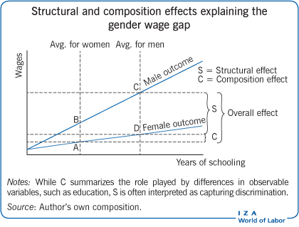
These two effects are summarized in the illustration on page 1, which is inspired by similar figures in [3], [4]. Wages are measured on the Y-axis and years of schooling on the X-axis. The wage structures for men and women are given by the blue lines. The market prices for years of schooling are given by the slopes of those lines. On the one hand, the structural effect is given by the difference between wages received by men and women if women had the same average educational level as men (the vertical distance between points D and C). On the other hand, the composition effect is given by the difference in average years of schooling between men and women priced at the female education level premium, i.e., the difference between the wage that, on average, a woman would earn if she had the same education level as the average man and the wage that she would earn if she had the average female years of schooling (the vertical distance between points A and D).
A numerical example may help to understand this scenario and the differences between structural and composition effects. Assume that the market pays $2 for each additional year of education acquired by a man, while it pays only $1 for each additional year of education acquired by a woman. Assume also that the average woman has 12 years of education, while the average man has 14 years of education. In this case, the overall effect (i.e. wage gap) is $16 (= 2 × 14 − 1 × 12), while the structural and composition effects are $14 (= [2 − 1] × 14) and $2 (= 1 × [14 − 12]), respectively. This is just a simplified example meant to illustrate the main concept. For a recent application of Oaxaca-Blinder Decomposition to the gender and racial wage gaps in the US, see [5].
There are decomposition methods that go beyond the mean, such as the RIF-Regression Decomposition, which is a regression-based tool, making it computationally easy to implement [6], [7]. Now, instead of looking only at the difference in mean wages of male and female workers, it is possible to examine the difference in each percentile of the distribution of male and female wages. A percentile is a measure indicating the value below which a given percentage of the population is in terms of its probability distribution. For example, the 20th percentile of the wage distribution is the wage value below which 20% of the population belongs. In other words, 20% of the worker population earns less than the 20th percentile of the wage distribution. Moreover, a percentile is an example of a quantile, which is a more general way to divide a given distribution into any number of partitions, not only percentages. As such, to examine the glass-ceiling effect, one would compare the 90th percentile, also known as the ninth decile, of the male wage distribution with the ninth decile of the female wage distribution. If interested in low-paying jobs due to poverty and social vulnerability concerns, comparing the tenth percentile, also known as the first decile, of the male wage distribution with the first decile of the female wage distribution would be relevant.
Moreover, for each percentile, it is possible to decompose the wage gap between men and women into its structural and composition effects, allowing researchers to provide the same interpretation for both structural and composition effects as in the usual Oaxaca-Blinder Decomposition. The richness of this procedure is exemplified by Figure 1. For each quantile, an estimation of the wage gap given by the overall effect is shown. Also visible are the structural and composition effects that capture, respectively, the differences in the wage structure between men and women and the differences in the distribution of observable variables between men and women priced at market values. Likewise, the glass-ceiling effect can be observed because the overall effect is larger for higher wages than it is for lower wages. Moreover, it is apparent that the glass-ceiling effect is explained by more intense discrimination (increasing structural effect), which compensates for smaller differences in observable variables (decreasing composition effect) at the top of the wage distribution. Finally, in this scenario, women are actually favored in the labor market for less-qualified jobs since the structural effect is negative for low wages.
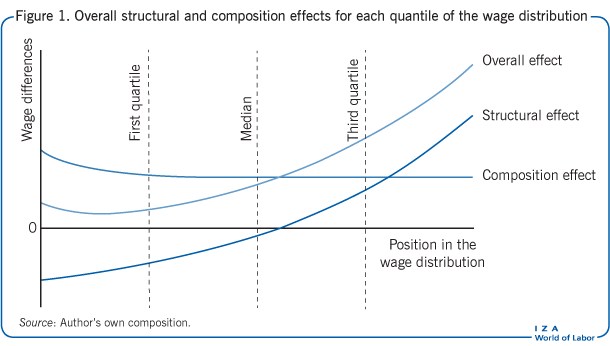
Figure 1 illustrates the concept. For a recent empirical example of an RIF-Regression Decomposition that discusses the racial/ethnicity wage gap under performance pay, see [8].
Decomposition methods can analyze precise segments of a population
There is one more advantage of the Oaxaca-Blinder and RIF-Regression Decomposition methods that has not yet been mentioned. They not only separate the overall effect into the structural and composition effects, but also decompose these two effects into smaller parts that are associated to each observable variable. For example, one piece of the structural effect is the difference in the labor market between the college premium paid to men and women and another is the difference in the job tenure premium paid to men and women. In a similar fashion, one piece of the composition effect is the difference in college attendance between men and women and another is the difference in lifetime work experience between men and women. A real-world empirical example, based on US data, is the best way to explain these detailed decompositions [9].
Figure 2 reports the decomposition results for the gender wage gap using the Oaxaca-Blinder Decomposition (column 1) and the RIF-Regression Decomposition (columns 4 to 6) when males are used as the reference group. On the first row, the Oaxaca-Blinder Decomposition shows that men earn approximately 26% more than women. Comparing the total structural effect and the total composition effect, it is clear that the latter is much more important in explaining the average gender wage gap, implying that differences in pay between men and women arise due to differences in their observable variables. More specifically, a woman with the same average characteristics as a man would earn 22% more than the average woman if both were paid like women. In particular, differences in lifetime work experience between men and women account for most of the gender wage gap. Since the structural effect is close to zero, a potential interpretation is of relatively little gender discrimination, at least on average. This first Oaxaca-Blinder-based analysis suggests that policymakers attempting to reduce the gender wage gap should, instead of intervening in the labor market, design policies that help women make career decisions more similar to the ones made by men, such as by creating public daycare centers, which would enable women to spend more time at work.
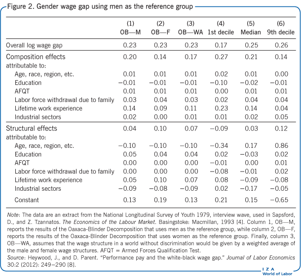
Interesting discoveries appear when comparing the RIF-Regression Decomposition results for the first decile, the median, and the ninth decile to the Oaxaca-Blinder results. Looking at the median, a very similar story emerges in this case compared to the one told by the first method's mean. However, the first and ninth deciles reveal a completely different picture. First of all, the evidence supports the existence of a glass-ceiling effect—the gender wage gap for top wages (ninth decile) is larger than the gender wage gap for low wages (first decile). Second, the composition effect is lower for top wages than for low wages, implying that ninth-decile female workers are more similar to their male counterparts than low-paid women are to low-paid men. In particular, women in the first decile of the wage distribution accumulate much less lifetime work experience than men, suggesting that poor women may have fewer options to reconcile their family and professional lives. Third, the structural effect presents extremely different behaviors for low and top wages. In the first decile, a woman is paid more than a man with the same observable characteristics, while, in the ninth decile, a woman earns much less than a similar man. This result suggests that, while there may be discrimination against women in top-paying jobs, women are actually favored in the labor market for less-qualified jobs. This result calls for a more complex policy intervention that would affect different female workers differently.
Restrictions to the decomposition method
Although decomposition methods are powerful statistical tools, they do have some important drawbacks. The most significant ones are related to the assumptions underlying them. In order to have a valid decomposition of the gender wage gap, unobservable variables that affect wages must be independent of gender and conditional on the explanatory variables that are considered in the regression analysis. For instance, if women anticipate that they will be discriminated against by employers, a selection process may occur with respect to ability, where only high-ability female workers take part in the labor market. In this case, the structural effect would be underestimated, because it would not account for female workers who do not even try to find work due to expected discrimination.
Moreover, when decomposing wage gaps, a reference group must be chosen. The reference group determines which wage structure to use to price differences in the distribution of observable variables and which value of the observable variables will be used to measure the differences in the wage structure. This choice does not affect the overall effect, but it affects the magnitude of the structural and composition effects. For instance, in the illustration on page 1, men were chosen as the reference group. If women had been chosen instead, the structural effect would be the vertical distance between points A and B, while the composition effect would be the vertical distance between points B and C. Compared with the initial choice of reference group, the composition effect would be larger and the structural effect would be smaller than initially measured. Following the previous numerical example, the composition effect would be equal to $4 (= 2 × [14 − 12]) and the structural effect $12 (= [2 − 1] × 12) when using women as the reference group (instead of $2 and $14, respectively, when using men as the reference). In the empirical example, column 2 of Figure 2 reports composition and structural effects of the gender wage gap when using females as the reference group. In this case, a large decrease of the former and a large increase of the latter effect is observed, suggesting that any possible discrimination may be more severe than initially imagined.
One possible solution for this statistical problem, also known as the “index problem,” is to compare studies that use the same reference group. In the literature on the gender wage gap, males are the most common reference group, as is the case in columns 1 and 4 to 6 of Figure 2. Another possible solution is related to the partial equilibrium nature of decomposition methods, since they do not take into account general equilibrium effects, which could be relevant as a consequence of labor market adjustments. In the above example, the question of what would happen to female wages if women were paid like men was posed. However, paying women and men equally may affect the male wage structure itself. In this situation, the currently observed male wage structure is a terrible approximation of the wage structure that would prevail if all workers were equally paid, thus biasing estimates of the structural effect. To handle this issue, one can assume that the wage structure that would prevail in a non-discriminatory world is a weighted average of the male and female wage structures [10], [11]. There are two common ways to choose the weights of this average: (i) using the population share of males and females [10]; or (ii) using a data-driven process based on the distribution of characteristics that yields a number in between those shares [11]. Results using the second option are shown in column 3 of Figure 2. By construction, these results are between those reported in columns 1 and 2. It is expected that these estimates are closer to the true composition and structural effects than the estimates from columns 1 and 2.
Another issue pointed out by decomposition methods’ critics is the interpretation of the structural effect. Decomposition methods do not have a causal interpretation because, strictly speaking, one can only discuss causal effects if the treatment can be manipulated. Since gender and race are immutable individual characteristics, the structural effect cannot be interpreted as any form of treatment effect. Consequently, decomposition methods can only be viewed as accounting exercises based on correlations.
Finally, it is tricky to interpret detailed decomposition results associated with categorical variables, such as industry sectors or education-level dummies. The problem is that the estimated detailed effects will depend on the choice of the omitted category. For example, if the education variable is categorical, such as low, medium, and high schooling levels, results may depend on which one of these three levels will serve as the reference. Thus, comparisons of different results will only be valid across studies that omit the same categorical variables. Another way to validly compare results is through aggregation. In the previous example, one would obtain a total effect due to education and not separate ones, such as the effect related to medium or high schooling levels. In fact, since the aggregated results for all categorical variables are not sensitive to the choice of omitted group, the researcher can easily focus on the effect of all education variables or the effect of all industry sectors, as done in Figure 2.
Limitations and gaps
Recently, there have been important theoretical developments linking decomposition methods to the large literature on program evaluation and treatment effects. The next important direction for future research is to improve the connection between decomposition methods and structural modeling. While standard decomposition methods can uncover the main forces underlying an economic phenomenon of interest, structural econometrics can be used to deepen understanding about the specific economics behind those forces, thereby providing insights into the black box of decomposition and structural effects.
It is important to mention that, although large structural effects are generally interpreted as evidence of discrimination in the labor market, those results could be generated by differences in unobservable variables between the two groups as well or by misspecification of the wage structure. In the example about gender wages used in this article, if unobservable variables that affect wages, such as ability, depend on gender then the estimated structural effect will be biased, invalidating its interpretation as evidence of discrimination. In the case of misspecification of the wage structure, using a different model for the lifetime work experience from the one used for the true wage structure may provoke large biases on the detailed structural effects, illustrating the dependence of decomposition methods on their linearity assumptions regarding the wage structure. Of course, this applies not only to the wage example but to any other outcome of interest.
Summary and policy advice
Discrimination in the labor market is a huge concern for policymakers. In this context, decomposition methods can cast new light on this problem by estimating discrimination's overall effect, and by decomposing it into two subcomponents: the structural effect and the composition effect. The relative importance of these effects can guide policies that aim to reduce inequality in the labor market. On the one hand, if there is evidence of discrimination in the labor market through large structural effects (i.e. built in bias against a certain population segment), then a policymaker may intervene directly by imposing financial penalties to discriminating firms.
On the other hand, if minority and majority groups differ in observable variables (which are encompassed within the composition effect), then a policymaker may want to design interventions to influence directly the decisions that affect those observable variables, such as new and innovative educational policies.
Acknowledgments
The author thanks two anonymous referees and the IZA World of Labor editors for many helpful suggestions on earlier drafts. Previous work of the author (together with Nicole Fortin and Thomas Lemieux) contains a larger number of background references for the material presented here and has been used intensively in all major parts of this article [9]. The author is also grateful to the superb research assistantship of Vítor Possebom.
Competing interests
The IZA World of Labor project is committed to the IZA Guiding Principles of Research Integrity. The author declares to have observed these principles.
© Sergio Pinheiro Firpo
Key terms for understanding decomposition methodology
Quantile: A quantile is a statistical concept used to describe the distribution of a random variable. The most famous quantile, known as the “median,” divides the distribution in a way that guarantees that half of the distribution of that variable is below the median and half is above the median.
Other famous quantiles, the first and ninth decile, divide the distribution in a way that guarantees that one-tenth or nine-tenths of the variable distribution is smaller than the first and ninth deciles, respectively. As a numerical example, imagine that you collect a sample of 10 individuals and observe values of 1, 2, 3, 4, 5, 5, 6, 7, 7, 8, 10 for some specific variable. In this case, the first decile, the median, and the ninth decile are 1, 5, and 10, respectively.