Elevator pitch
Randomized control trials are often considered the gold standard to establish causality. However, in many policy-relevant situations, these trials are not possible. Instrumental variables affect the outcome only via a specific treatment; as such, they allow for the estimation of a causal effect. However, finding valid instruments is difficult. Moreover, instrumental variables (IV) estimates recover a causal effect only for a specific part of the population. While those limitations are important, the objective of establishing causality remains; and instrumental variables are an important econometric tool to achieve this objective.
Key findings
Pros
Valid instrumental variables help to establish causality, even when using observational data.
Using instrumental variables helps to address omitted variable bias.
Instrumental variables can be used to address simultaneity bias.
To address measurement error in the treatment variable, instrumental variables can be used.
Cons
Finding strong and valid instrumental variables that affect participation in the treatment but do not have a direct effect on the outcome of interest is difficult.
Estimated treatment effects do not generally apply to the whole population, nor even to all the treated observations.
Estimated treatment effects may vary across different instruments.
For small sample sizes, and in case of “weak” instruments, instrumental variable estimates are biased.
Author's main message
When treatment is not randomly assigned to participants, the causal effect of the treatment cannot be recovered from simple regression methods. Instrumental variables estimation — a standard econometric tool — can be used to recover the causal effect of the treatment on the outcome. This estimate can be interpreted as a causal effect only for the part of the population whose participation in the treatment was affected by the instrument. Finding a valid instrument that satisfies the two conditions of (i) affecting participation to the treatment, and (ii) not having a direct effect on the outcome, is however far from trivial.
Motivation
Instrumental variables (IV) estimation originates from work on the estimation of supply and demand curves in a market were only equilibrium prices and quantities are observed. A key insight being that in a market where, at the same time, prices depend on quantities and vice versa (reverse causality), one needs instrumental variables (or instruments, for short) that shift the supply but not the demand (or vice versa) to measure how quantities and prices relate. Today, IV is primarily used to solve the problem of “omitted variable bias,” referring to incorrect estimates that may occur if important variables such as motivation or ability that explain participation in a treatment cannot be observed in the data. This is useful to recover the causal effect of a treatment. In a separate line of enquiry, it is demonstrated that IV can also be used to solve the problem of (classical) measurement error in the treatment variable.
Discussion of pros and cons
Advantages of using instrumental variables to demonstrate causality
As an example, consider the issue of estimating the effect of education on earnings. The simplest estimation technique, ordinary least squares (OLS), generates estimates indicating that one additional year of education is associated with earnings that are 6–10% higher [2]. However, the positive relationship may be driven by self-selection into education, i.e. individuals who have the most to gain from more education are more likely to stay. This will be the case, for example, if pupils with higher ability find studying easier, and would likely receive higher wages anyway. As such, the positive correlation observed between years of education and wages would partially reflect the premium on ability and could not be interpreted as the returns from an additional year of education, as intended. OLS estimates would thus not be informative about the effect of a policy designed to increase years of education. This problem is called “omitted variable bias.” It occurs when a variable (such as ability) that is not observed by the researcher is correlated both with the treatment (more education) and with the outcome (earnings). The direction (over- or underestimation) and size of the bias in OLS estimates is a function of the sign and strength of the correlations.
In this example, a randomized control trial (RCT), which would entail allocating education randomly to individuals and observing the differences in their wages over their lifetime, is simply not feasible on ethical grounds. However, some natural or quasi- natural experiments can come close to altering educational choice for some groups of individuals, and as such, can be used as instruments. One such natural experiment is a change in the legal minimum age at which pupils may leave school (school leaving age). This type of change affects all pupils, independent of their ability. It therefore acts like an external shock that cannot be influenced by the individual student.
Numerous countries have legislation stipulating the age at which pupils can leave the educational system. For example, say that a child can leave school on the last day of the school year if she is 14 by the end of August. Assume now that the legislation is altered, so that children have to be 15 by the end of August to be allowed to leave school. Children who wanted to leave school at 14 are prevented from doing so, and have to remain for an additional year of schooling. Under the (strong) assumption that children under the two legislations are similar and face similar labor markets conditions, the legislation change creates a quasi-natural experiment: independently of their ability, some individuals will be affected by the change in school leaving age and have to remain for an additional year of schooling, while pupils with similar preferences from the previous cohort will not. If researchers knew who wanted to leave school at 14, they could compare the outcomes of individuals who left school at 14 to the outcomes of individuals who were forced to stay until 15. This simple difference would then be the causal effect of remaining in school between the ages of 14 and 15. Unfortunately, observational data do not allow to identify individuals whose educational choice was affected by the reform; so, under the new legislation, individuals who wanted to leave school at 15 are indistinguishable from those who wanted to leave at 14 but had to remain for another year. What the reform does, nonetheless, is to alter the probability of staying in school, and can thus be used as an instrument as it affects the probability of treatment (another year of schooling) without affecting the outcome of interest (e.g. earnings).
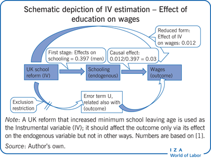
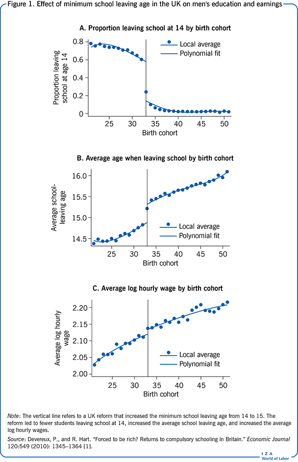
In 1947, a legislative change in the UK increased the minimum school leaving age from 14 to 15, affecting children born in 1933 and after. This change in the law provides an opportunity to evaluate the effect of (additional) schooling on earnings [1]. In Figure 1, panel A shows that the reform affected both the fraction of children leaving school at the earliest opportunity and panel B refers to the total amount of schooling completed. Estimates indicate that the reform increased the average years of schooling for men by 0.397 years. This estimate of the effect of the reform (the IV) on the treatment (education) is known as the “first-stage regression.” If education has any causal effect on earnings, the average earnings of individuals affected by the reform should also be higher. This is indeed the case as shown in panel C of Figure 1, which reports the average log earnings for men. This series shows a clear break in 1933, the magnitude of which implies that individuals affected by the reform earn, on average, 1.2% higher wages. This second estimate of the effect of the reform (the IV) on the outcome (earnings) is known as the “reduced form estimate.” A simple IV strategy, in this case using a binary instrument that takes on only two values (1 for being affected by the reform, and 0 for not being affected by the reform), is the ratio of the reduced form estimate over the first stage estimate. (This ratio is also known as the Wald estimate.) In this case the causal effect of additional education on earnings would be 0.012/0.397 = 0.030 and thus about 3%.
The intuition of this approach is that the effect of one more year of education on wages is basically the effect of the reform (the IV) on wages (the outcome) — which is given in the reduced form—scaled up by the effect that the reform has on years of education (the treatment) — which is what the first stage estimate is about. If the instrument is “relevant,” i.e. has an effect on education (the treatment), and if the instrument affects wages “exclusively” through its effect on education, then the IV estimates can be interpreted as the causal effect of the treatment on the outcome. These two conditions are called “instrument relevance” and “exclusion restriction.”
To summarize, when an unobserved variable such as ability correlates both with the treatment and the outcome, a simple estimate like OLS will be biased due to self-selection into the treatment. Similarly, if the treatment variable is measured with error, the OLS estimate will be biased toward zero. However, a causal estimate of a treatment on an outcome can be recovered if a credible instrument can be found. A credible instrument must satisfy two conditions:
- Relevance: the instrument must affect the probability of treatment. In a regression of the treatment on the instrument, also known as the first stage equation, the coefficient on the IV must be sufficiently strong.
- Exclusion restriction: the instrument affects the outcome exclusively via its effect on the treatment.
If such an IV can be found (i.e. both relevance and exclusion restriction are fulfilled), then an IV strategy can be implemented to recover a causal effect of the treatment on the outcome.
The previous example presented the Wald estimate, i.e. the ratio of estimates from two regressions: the reduced form estimate, coming from a regression of the outcome on the instrument; and the first stage estimate, coming from a regression of the treatment on the instrument. This can easily be computed when the instrument takes only two values. In the more general case, a so-called “two stage least squares” (2SLS) estimate will be computed, whereby predictions of the treatment from the first stage equation are used in a regression of the outcome on the treatment, rather than the true value of the treatment. As such, only the variation in the treatment coming from the instrument is used to explain the variance in the outcome. This then solves the self-selection bias. In the case of a binary (two-value) instrument, the Wald and 2SLS estimates will be identical (see [3], for example). However, the difficulty is not in the implementation of such a 2SLS estimate, all statistical packages can compute IV estimates, but in (a) finding a valid instrument and (b) interpreting the results. The discussion will now focus on these two points
Finding a valid instrument
To understand the search process for a valid instrument, the two necessary conditions mentioned above (relevance and exclusion restriction) must be met. To satisfy the first condition, the correlation between the instrument and the treatment allocation must be strong. Weak instruments, those which are only weakly correlated with the treatment, do not solve the omitted variable bias of OLS estimates and in severe cases can bias estimates even more significantly [4]. Methods for detecting and dealing with weak instruments are discussed below.
The second condition (exclusion restriction) for a valid instrument is that the instrument affects the outcome exclusively via its effect on the treatment. Unfortunately, this condition cannot, in general, be statistically tested. It is exactly for this reason that finding a valid instrument is so difficult. Here, econometrics cannot escape economics: Econometric analysis needs to be supported by a convincing economic narrative, which provides credibility to the exclusion restriction. Following our example, one may believe that the change in minimum school leaving age had no direct effect on earnings. However, if assuming that young and old workers are not very good substitutes, employers wanting to recruit 14-year-old workers in 1947 would have faced a severely reduced supply of such workers and may have had to subsequently increase wages in order to recruit new employees. If starting wages have long-term effects on career development, one could argue that the change in school leaving age is not a good instrument, because the higher starting wage of the few 14-year-olds who left school despite the increased school leaving age would lead to higher wages throughout their career independently of their schooling. However, since worker substitutability is likely to be high, such concerns are probably limited. Yet, the argument shows that instrument validity is not a given but depends on the context.
Nonetheless, there are several important examples of instruments that have been used widely in applied literature. It must be stressed that there are no "free lunches" and none of the commonly used IVs will be applicable in every setting. It is the task of the researcher to identify relevant sources of exogenous variation and specify their instrumental variable accordingly.
Unexpected policy changes - as illustrated by the previous example, public policy changes can often be a source of promising instruments since they affect the allocation to treatment independently of preferences, like in an RCT. For a policy change to be used as an instrument, it must not have been announced too far in advance of implementation, to ensure that allocation to the treatment is as close to being random as possible. Often unexpected policy changes will generate a cut-off date or (monetary) value around which there is a jump in the probability of receiving treatment. Since this cutoff is relevant to the treatment and generated from an exogenous policy change, it can be used as a valid instrumental variable. One limitation of this approach comes from the fact that the cutoff only affects a subset of individuals that are sufficiently close to it, hence any causal statements are only locally valid.
Lottery – like public policy interventions, participation in treatment is sometimes determined via a lottery or a similar quasi-random process. The simplest example is a military draft where individuals are randomly selected into military service or are randomly given the opportunity to join a training program. In either case, the lottery number of the individual can be used as an instrument for participation. However, when using this instrument, it is crucial to distinguish between its ignorability and exclusion. The former implies that the assignment of the instrument to each unit is not correlated with other unobserved determinants of the outcome, while the latter adds that there are no direct or indirect effects of the instrument on the outcome except its effect on the endogenous regressor. Ignorability is satisfied mechanically due to the randomization process, while exclusion remains open to challenge: even though individuals are randomly selected into military service, receiving a draft letter may encourage non-compliant behaviour such as staying in school or moving abroad that alter outcomes of interest [5]. However, such an outcome would violate the exclusion restriction as these will impact the outcome through channels other than the treatment.
Bartik shift-share - predicts a region-level outcome by interacting a set of aggregate-level shocks (shifts) with region-specific weights (shares). As with any instrument, some component of this decomposition must be “as-good-as-randomly” assigned to units. In exposure designs, it is common to assume that this exogenous variation comes from the allocation of the shares between units. Classic examples of this approach are studies of the impact of immigration on the wages of natives. Since immigrants settle in areas where their ethnic community is largest, the shift-share instrument is constructed by interacting past settlement shares of different ethnicities with total national inflows of these different migrant groups. Crucially, this instrument relies on the strict exogeneity of shares conditional on observable characteristics of each region. This implies that these shares are not correlated with changes in unobserved determinants of the outcome of interest. In the case of migration, this would mean that for regions with similar characteristics, it is only the “pull-factor” of having a large pre-existing ethnic community that explains differences in migration patterns. A simple way of testing this is by checking whether regional characteristics that are correlated with initial shares suggest other channels through which these shares may affect the outcome. Other diagnostic checks are suggested in a recent study [6]. Alternatively, if there are many independent exogenous shocks or shifts, even if shares have been allocated endogenously, it is possible to recover a consistent estimate for the treatment effect. It must be emphasised that since shocks occur at a more aggregate level, to avoid bias, there must be numerous channels, such as industries, through which the shocks affect each region. Only then can the bias cause by non-random exposure be “averaged out” [7].
Judge/examiner designs – leverage the random assignment of individuals to a set of decision-makers who differ in their “leniency” with respect to the assignment of a treatment. For instance, when defendants are randomly assigned to judges who have different sentencing propensities, it becomes possible to use this design to instrument for incarceration. As these judges or decision-makers are typically randomly assigned, this IV often has considerable a priori credibility. Nonetheless, caution must be taken when using this design as strategic decisions from the defendant utilizing information about the reputation of the assigned judge may lead to violations of the exclusion restriction as it requires that the instrument affect the outcome exclusively through the decisions of the official. Moreover, as will be discussed below, the validity of estimates can be undermined if the assumption of monotonicity is not met: an instrument violates this assumption if its impact on the propensity to receive treatment is positive for some units and negative for others. In this case, this means that for some subgroups of defendants, harsher judges occasionally pass more lenient sentences. A recent study has proposed a test for both conditions [8].
Weather shocks – use unexpected changes in weather conditions such as rainfall or extreme temperatures to predict either the timing of a treatment or individual decisions. Weather-based instruments are attractive because meteorological conditions are unaffected by human behavior and influence decision-making through a small set of channels. Hence, these instruments have been used widely to study economic growth, migration, crime and even political activism. Even so, care must be taken when justifying the exclusion restriction for this IV. For example, when studying the relationship between conflict and income in developing countries, it was common to use rainfall as an instrument for income. Relevance can be guaranteed by the fact that many such economies have large agricultural sectors whose profits are highly sensitive to changes in crop yields that in turn depended on the weather. Unfortunately, a study on this relationship in India found that areas in which rainfall had no effect on income still saw differences in conflict intensity that depended on the quantity of rainfall. The general lesson is that factors like rainfall may have far-reaching effects outside of the treatment channel [9].
It is often desirable to test the plausibility of the assumptions underlying a given IV design and though each situation is unique, several methods have been suggested that can provide support to both the relevance and exclusion restrictions. As opposed to some tests discussed above, these approaches are not limited to a specific design.
Assessing the relevance condition for an instrument involves verifying that the correlation between the instrument and endogenous variable is sufficiently strong. If this relationship is weak, the approximate normality of the estimated coefficients breaks down undermining inference in both stages of IV estimation. These problems have led to the development of formal testing procedures for weak instruments based on the first-stage F-statistic (a value that helpsto asses the strength of the instruments), as well as the derivation of identification-robust confidence intervals. In practice, when errors of the regression are homoscedastic (that is their variance is constant), it is reasonable to follow the well-known “rule-of-thumb” that the F-statistics should be around 10 to rule out weak instruments [10]. However, homoscedasticity assumptions are often implausible. The case of non-homoscedastic errors is more complex, and researchers are often insufficiently careful with what statistics are reported. Worryingly, many papers only report the Kleibergen-Paap Wald statistic which has little theoretical justification in case of weak instruments [11]. Instead, where only one endogenous regressor is present, it is recommended to calculate the effective (Olea-Pflüger) F-statistic. Cases with multiple endogenous regressors are still an active area of research; for more details on these tests, see the recent review [11].
At this stage it is important to ask: what does a researcher do if a weak instrument has been detected? It seems intuitive to simply drop the weak instrument and search for a new one. However, on aggregate, this results in publication bias as well as distortions to the size of published tests [11]. Unfortunately, this is often unavoidable as conclusions based on weak instruments are difficult to publish in the first place. To an extent, this can be alleviated by using tests that are valid even in the presence of weak instruments. Of these, the most prevalent is the Anderson-Rubin test, which is unbiased and, in the just-identified case, has higher statistical power than any unbiased alternatives. Moreover, it has higher power to detect negative effects even if instruments are strong! For this reason, the authors of one study argue that it should replace the 2SLS t-test altogether! For more details on the problems of inference under weak instruments see [12].
Evaluating the exclusion restriction is more difficult. Nonetheless, two approaches have been suggested that allow researchers to detect or test sensitivity of estimates to mild violations of this restriction. Firstly, one can rerun the reduced-form regression on a subgroup of the population for whom the first stage regression coefficient is zero. If this approach yields a significant coefficient, then it means that the instrument affects the outcome of interest through channels other than the treatment [13]. For example, in studying the impact of compulsory schooling laws in the 20th century, it was common to use quarter-of-birth as an instrument for being affected by the policy. However, it was later found that men born earlier who were un-affected by schooling laws still exhibited differences in earnings by their quarter-of-birth. This implies that quarter-of-birth impacts the earnings not only via an individual being affected by the law but also through other means [4], [14]. This therefore provides strong evidence against the validity of the exclusion restriction.
Secondly, researchers can test the sensitivity of their IV results by making assumptions about either the range or distribution of possible direct effects that an instrument may have on the outcome of interest. Following the example above, some studies have found that the direct effect of quarter-of-birth on wages is approximately 1%. Hence, by re-estimating the IV model and varying the violation of the exclusion restriction around this effect size, it becomes possible to derive adjusted confidence intervals for the estimated IV coefficient that reflect how sensitive this result is to failures of the exclusion condition [14].
Interpreting IV estimates: The Local Average Treatment Effect (LATE)
Assuming that a valid instrument has been found, the remaining difficulty is the interpretation of the IV estimate. Going back to our example of the returns to years of education in the UK, the IV estimate obtained from using the change in school leaving age was 3% higher wages, only about half the OLS estimate. What could explain this much lower estimate of the returns? The probable answer is that the OLS estimate suffers from omitted variable bias if, for instance, information regarding ability is unobservable. Since ability is positively correlated with both years of education and earnings, its omission from the OLS regression means that the effect of ability on earnings is picked up by the education variable, overestimating the direct effect of education on earnings (upward bias). However, the literature reports several cases of IV estimates of the returns to education that are greater than the OLS estimate (see the review in [2]), how is this possible? One reason is that education is often measured with error, especially in surveys, and that this measurement error in the treatment biases the OLS estimate of the treatment effect toward zero (OLS estimates are “too small”). Since the IV estimate is unaffected by the measurement error in the treatment variable, they tend to be larger than the OLS estimates. However, the main reason why the IV estimate might be larger than the OLS estimate, even in cases were the omitted variable bias is expected to be the other way round, is that while the OLS estimate describes the average difference in earnings for those whose education differs by one year, the IV estimate is the effect of increasing education only for the population whose choice of the treatment was affected by the instrument (in our example, those 14-year-olds forced to stay in school an additional year who would not otherwise have). This is known as the “local average treatment effect” (LATE). Economic theory predicts that the marginal returns to education (return to one additional year of schooling) decrease with the level of education: so, learning to read has very high returns, but doing a PhD might not do much to increase earnings. This concept is made clearer in Figure 2. At low levels of education (below the average level S*), the return to one additional year of education is greater than the average return (r*). The reverse is true at higher (above average) levels of education. These decreasing returns to education are important when trying to understand why the IV estimate may be larger than the OLS estimate, even in a case where OLS estimates are expected to be upward biased due to omitted variable bias.
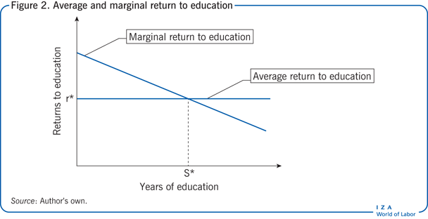
The assumption now is that the instrument affects the educational choice of low achievers. The IV estimates indicate a positive effect of additional education for low achievers (below average, left of S* in the figure); for this group, the returns are even greater than for the average population. The situation is reversed when examining an instrument that affects high achievers (i.e. for people with above average education the IV estimate might be lower than the OLS estimate). As such, while it is possible to have one OLS estimate of the returns to education for a given population, different instruments will yield different IV estimates of the returns to education specific to the group affected by the instrument. Rephrasing this statement, it can be said that IV estimates have strong “internal validity” (for specific groups) but may have little “external validity” (for the entire population): in our example, the IV recovers the returns to one additional year of education for individuals who wanted to finish school at age 14 in 1947, but were forced to stay for an additional year. This return might be very different from the return to one additional year of education for other cohorts or individuals with a greater taste for education, i.e. one additional year of education later on in life. While this interpretation of the IV estimate may appear very restrictive, it is in fact similar to the Interpretation of an RCT, for instance.
The difficulty in interpreting an IV estimate as a local characteristic (i.e. LATE) is that it is not possible to formally identify the individuals whose decision to participate in the treatment was affected by the instrument. Formally, in the case of a binary treatment (cohorts that are affected by the new higher compulsory schooling age, in contrast to cohorts born before 1933 and thus unaffected by the reform) and a binary instrument (school attendance until at least the age of 15, or school attendance only until the age of 14 or less), the population can be divided into four groups, as shown in Figure 3.
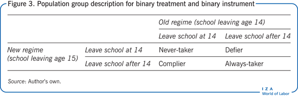
Every student can only be one of four types. “Always-takers” are those who leave school at age 15 or above, independently of whether the compulsory schooling age is 14 or 15. “Never-takers” leave school at age 14, independently of whether the compulsory schooling age is 14 or 15; in the example, this group ignores the new legislation and drops out of school anyway. “Compliers” are students who leave school at age 14 when the compulsory schooling age is 14, but they continue to age 15 when the compulsory schooling age is 15. “Defiers” are students who leave school at age 15 or older even when the compulsory schooling age allows them to leave at age 14, but when the compulsory schooling age is 15, they drop out earlier. “Defiers” do the exact opposite of what the law prescribes: less if more is asked, and more if less is asked.
To be able to interpret an IV estimate as a LATE, an additional assumption must be made on the instrument: monotonicity [15]. The monotonicity assumption states that the instrument pushes some people from no-treatment into taking the treatment (compliers) but nobody in the opposite direction (defiers), i.e. individuals who react to the instrument at all do so in one (intuitive) direction only.
Accordingly, the IV is only informative about the effect of the treatment on the compliers but cannot identify the effect on always-takers and never-takers, since for these two groups, the treatment choice is unaffected by the instrument (they leave school at 14 or after age 14 independently of the reform). As such, the IV can recover the average treatment effect (the average effect of the treatment on the population) only if the always-taker and never-taker groups are very small and thus (statistically) negligible.
It is noteworthy that some recent studies have derived weaker conditions than monotonicity that preserve the validity of LATE interpretations of IV estimates [16]. Formally, this weaker condition requires that there exists a subgroup of the population of compliers that accounts for the same percentage of the total population as the defiers and has the same LATE. This condition holds if in each subgroup of the population which has the same value of the LATE, there are more compliers than defiers. In binary treatment designs, this holds when the sign of the LATE of the defiers is the same as the sign of the 2SLS coefficient. An interesting example where this is relevant is estimating the effect of incarceration on high-school completion rates [17]. Often such designs use the leniency of randomly assigned judges as an instrument for incarceration. The problem is that unless harsher judges always give out longer sentences than more lenient judges, the instrument will generate defiers. Fortunately, regardless of the length of the sentence, the effect for both compliers and defiers will have the same sign. Hence, a LATE interpretation is preserved
Limitations and gaps
While IV estimates are very helpful tools to measure causal effects, they are not beyond controversy.
A major criticism of IV is that it is often difficult to rule out violations of the exclusion restriction. Though it was shown how specific methods can be used to assess the influence of “mild” violations via restrictions on parameter estimates, researchers often under-estimate the potential number of alternative causal pathways from the instrument to the outcome of interest. This has been a particular problem in studies of economic growth where instruments such as legal origins or population growth have been used for multiple endogenous variables (e.g. financial intermediation, years of schooling or constraints on executive power), all of which are potential determinants of growth [18]. A similar issue has been observed in micro-level studies relying on weather-based instruments or more generally on “natural experiments”. A further difficulty is that reuse of the same source of exogenous variation generates a “multiple testing problem” where the rate of false positives found through hypothesis testing is much higher than the commonly used cutoff of 5% [19]. These concerns highlight the need to give detailed economic justifications of the exclusion restriction supplemented by the relevant diagnostic/sensitivity tests.
Moreover, as mentioned before, different instruments will identify treatment effects for different subgroups, and will therefore lead to numerically different treatment effects. This can also be considered good news if one looks at several different instruments that are informative about treatment effects for different sets of compliers. This point is nicely illustrated in the literature by looking at two different instruments for the same treatment (schooling) [20]. In this example, the first instrument is whether a child attending school during the WWII had a father engaged in the war. The second instrument is the father’s education. The father-in-war instrument is likely to (negatively) affect the schooling of smart children who are constrained because of their father’s absence from home. The father’s education instrument builds on an intergenerational correlation of education: smarter fathers can help their children get smarter. Having a smart father (as opposed to not) might make more of a difference for the schooling of rich children who are not very smart to begin with. These two instruments affect complier groups at opposite ends of the “returns to schooling” spectrum: the first one should recover the returns for individuals with low levels of schooling (their schooling was reduced due to the absence of the father), while the second identifies the returns for individuals with high levels of education [20]. IV estimates find that the returns to schooling are between 4.8% per year for the father’s education IV and 14.0% per year for the father-in-war IV, showing a considerable heterogeneity in returns to schooling (as expected from Figure 2) [20].
Finally, it is necessary to highlight an additional limitation of IV, which is a bit more on the technical side: IV is consistent but not unbiased. Consistency means that, as estimation samples get larger and larger, IV estimates will converge to the “true” population parameter. Unbiasedness means that, even in finite samples, on average, if drawing a series of independent samples from the same population, would lead to the “true” population parameter. So, the fact that IV is consistent, but not unbiased is troublesome, because any sample is finite. In small samples, IV estimates are unlikely to recover the true effects, and will thus suffer from small sample bias.
Summary and policy advice
Taxpayers support public policies with their own money and have a right to know whether their money is well-spent. Politicians have warmed up to the idea that public policy interventions need to be seriously evaluated. While RCTs are a promising avenue to study the causal effect of treatments on outcomes of interest, they cannot be universally applied to all relevant policy issues. Methods dealing with observational data are thus important, and IV estimation has been a workhorse for empirical research over the last decades. However, finding valid instruments is not easy. Instruments need to fulfil two crucial conditions: they need to be relevant, i.e. significantly correlated with the treatment of interest; and they need to satisfy the exclusion restriction, i.e. they should only affect the outcome via their effect on the treatment. The first condition is testable, but a weak correlation between instrument and treatment is not good enough. Thus, instruments should be sufficiently strong because, otherwise, IV is no better than standard OLS regression. The second condition is fundamentally untestable. The possibility that an instrument affects the outcome above and beyond its effect on the treatment can never be excluded. It is this point that makes IV estimation a matter of debate and controversy. These debates are not merely academic; they are, in fact, crucial if researchers and policymakers are keen to avoid drawing wrong inferences about the direction and size of treatment effects. Nevertheless, with a good instrument, it is possible to get reliable estimates of treatment effects that can help influence effective policy.
Acknowledgments
The authors thank two anonymous referees and the IZA World of Labor editors for many helpful suggestions on earlier drafts. The authors also thank Wiji Arulampalam, Clément de Chaisemartin, Arnaud Chevalier, Andreas Ferrara, and Fabian Waldinger.Version 2 of this article updates the discussion of valid instruments, its interpretation and limitations. It adds a new Further reading and new Key references [6], [7], [8], [9], [11], [12], [13], [16], [17], [18], and [19] as well as Additional references.
Competing interests
The IZA World of Labor project is committed to the to the IZA Guiding Principles of Research Integrity. The authors declare to have observed the principles outlined in the code.
© Grigory Aleksin and Sascha O. Becker