Machine learning for causal inference in economics

Elevator pitch

Machine learning (ML) improves economic policy analysis by addressing the complexity of modern data. It complements traditional econometric methods by handling numerous control variables, managing interactions and non-linearities flexibly, and uncovering nuanced differential causal effects. However, careful validation and awareness of limitations such as risk of bias, transparency issues, and data requirements are essential for informed policy recommendations.

Key findings

Author's main message

ML provides structured, data-driven tools that reduce the need for discretionary decisions in model specification, such as selecting control variables or defining functional forms. It is particularly useful for handling large sets of control variables and capturing complex interactions, improving the precision of policy effect estimates. Additionally, ML can systematically identify differential effects across groups, offering valuable insights for policy design. However, its effectiveness depends on the quality of input data and the appropriate selection of model parameters to minimize bias and overfitting. For evidence-based policy recommendations, researchers and policymakers need to be aware of the limitations of ML to ensure that its findings are properly interpreted and applied.

Motivation

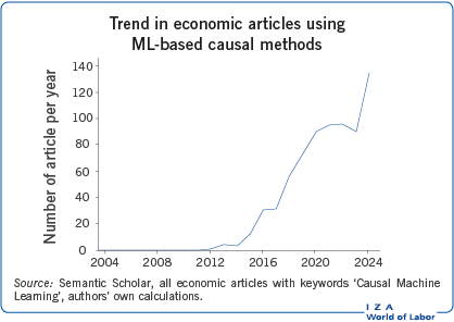
Machine learning (ML) has long been recognized for its predictive power, but its application to causal inference - known as Causal ML (pioneered by [1]) - has only recently gained attention, as illustrated above. In economics, understanding the causal effects of policies and interventions is essential for informed decision-making. Causal ML methods provide tools to address challenges posed by modern data, such as managing a (very) large number of control variables and accounting for complex, non-linear relationships in big data. While Causal ML methods are not without limitations, they offer researchers and policymakers the ability to analyze the impacts of policies and interventions systematically, including uncovering differential impacts across groups. This article reviews how Causal ML can contribute to economic policy analysis by providing a structured and data-driven approach to understanding causal effects.

Discussion of pros and cons

Machine learning methods

ML offers tools for analyzing large, complex data sets, systematically accounting for important variables, and processing diverse data types such as text and images. This can provide information and recommendations for more effective, evidence-based policy making. ML also enables innovative applications, such as analyzing social media or customer reviews to identify trends or using satellite imagery to monitor environmental changes such as deforestation. Before discussing the specifics of Causal ML, some fundamental ML concepts and methods are introduced.

Overfitting

Overfitting occurs when a model becomes too closely tailored to its training data, capturing specific details and noise rather than identifying general patterns applicable to new, unseen data. For example, a model predicting stock prices might perfectly match historical trends but fail to predict future prices because it models random fluctuations rather than meaningful patterns. It is similar to a student who memorizes mock exam answers but struggles with slightly different questions in the actual test.

Unlike traditional econometric methods, which often do not systematically address overfitting, ML actively addresses this problem using resampling techniques such as cross-validation. Cross-validation partitions the data into subsamples, trains the model on some subsamples, and tests it on others. This sample partitioning acts as a firewall between the training and test samples, ensuring that the model performs consistently across subsamples and avoids being overly tailored to any specific subsample. This balances the so-called bias-variance trade-off: overly simple models (high bias) may miss important data patterns, while overly complex models (high variance) may overfit the data. By addressing this trade-off, cross-validation improves the ML model's ability to make predictions on new data.

Supervised machine learning

Supervised ML plays a key role in combining ML with causal inference, as it focuses on building predictive models where both inputs (e.g. control variables) and outputs are observed. Its main goal is to predict outcomes accurately from input data. Other ML methods include unsupervised learning and reinforcement learning. Below, some popular supervised ML methods are summarized:

• Lasso regression (least absolute shrinkage and selection operator) is a regularization technique for regressions, that prevents overfitting by shrinking some coefficients to zero, effectively excluding variables with low predictive power from the model. This makes it particularly valuable in high-dimensional datasets, with more control variables than observations, where traditional methods cannot be applied. By retaining only the most predictive control variables, Lasso balances model complexity and generalizability. However, it performs best in sparse models, where only relatively few variables are good predictors, and may have a lower predictive performance when many variables are equally relevant for prediction. For example, in wage prediction, Lasso might prioritize factors like education and experience while excluding less predictive ones, such as workplace perks.
• Decision Trees partition data into branches based on rules derived from input variables. They subsequentially split samples by selecting the variable and threshold that minimize prediction error at each step. Each branch ends in a leaf, with the average outcome in the terminal leaves representing the model's predictions.  Decision Trees are useful for modeling non-linear relationships and interactions but can be sensitive to small changes in the data. For example, when predicting loan default risk, a Decision Tree might classify borrowers into risk categories using splits based on income, credit score, and debt-to-income ratio. However, slight variations in the sampling procedure can lead to different tree structures, reducing the model's stability and interpretability.
• Random Forests are ensembles of Decision Trees that improve prediction accuracy and stability by aggregating predictions from multiple trees. Each tree is trained on a random subset of data and input variables, introducing diversity to the trees. The final prediction is obtained by averaging the predictions of all trees, a process known as Bagging (Bootstrap Aggregation), which helps reduce overfitting. While Random Forests typically outperform individual Decision Trees in predictive power, they still lack interpretability. For example, in healthcare, Random Forests can effectively predict disease risks using data such as age, medical history, and genetic markers. However, the model's predictions are derived from potentially thousands of Decision Trees, making it challenging to interpret how specific factors influence the results.
• Neural Networks are advanced models inspired by the human brain, consisting of interconnected layers of nodes (neurons). Input data is processed through weights and non-linear mathematical functions (e.g., Sigmoid) within these layers to uncover patterns and relationships. They are particularly effective at capturing complex, non-linear relationships, making them ideal for tasks like image recognition and natural language processing. This makes them especially suited for analyzing unstructured data, such as text and images. However, Neural Networks require large datasets and substantial computational power for training. Their complexity also makes them "black boxes," as the model's inner workings are not easily interpretable. For example, they are foundational to large language models like ChatGPT, which have gained popularity for their ability to generate coherent text and answer questions.

Causal machine learning

Causal ML builds on Supervised ML to analyze cause-and-effect relationships rather than focusing solely on predictive patterns in data. While traditional econometric methods provide robust tools for causal analysis, Causal ML is particularly useful when working with datasets that contain (very) many control variables and complex, non-linear relationships. For example, in health policy, Causal ML can incorporate factors such as socioeconomic status, access to healthcare, lifestyle choices, and genetic predispositions - variables that are often highly correlated and challenging to model with traditional approaches alone. Causal ML can help to address two important challenges in policy analysis:

Accounting for confounders: Accounting for confounders - control variables that influence both the intervention (e.g., education) and the outcome (e.g., wages) - is critical for reducing omitted variable bias in many applications. However, including all available control variables can lead to overfitting and imprecise estimates of policy effects, particularly when datasets contain many control variables relative to the sample size. Causal ML offers tools to address this challenge by accounting for relevant confounders only, aiming to balance model complexity and accuracy while maintaining unbiased and precise estimates of policy effects.

Uncovering differential impacts: Causal ML can systematically identify how different groups respond to policy interventions at a granular level. This capability complements traditional methods by providing more detailed insights. It can help improve policy design, enable targeted implementation, and support efficient resource allocation.

Accounting for confounders

Accounting for confounders is critical not only in multivariate regression and matching estimation but also in instrumental variable (IV) analysis and difference-in-differences (DiD) approaches. For example, in IV analyses, the validity of an instrument may depend on controlling for specific confounders, while in DiD studies, the common trend assumption may require conditioning on relevant variables. Causal ML offers systematic tools to address confounders across all these methods, reducing reliance on discretionary decisions and incorporating interactions and non-linear relationships to fully account for confounding.

Use case: Earnings equation

The Mincer earnings equation is a canonical model in labor economics used to estimate the returns to education. It expresses earnings as a function of years of education, work experience, and tenure, with an additional error term accounting for other unobserved factors. The key focus is on the returns to education, while the other factors help capture additional influences on earnings.

However, real-world relationships between earnings and these factors can be more complex. To better account for these complexities, the model can be extended by including interaction terms and non-linear effects. For example, the impact of experience and tenure may not be purely additive but may interact with each other, and their effects may also change at different levels due to non-linearity.

Determining the most accurate model for estimating the returns to education is challenging. If important interactions or non-linear patterns are overlooked, the estimates may be biased due to model misspecification. On the other hand, including too many variables, especially in small samples, increases the risk of overfitting. This creates a trade-off between bias and variance. To address this challenge, Double ML, a specific Causal ML approach, can be used to balance the bias-variance trade-off and improve estimation accuracy in the earnings equation.

Double machine learning

Double ML isolates causal relationships by accounting for relevant controls and using flexible Supervised ML algorithms to mitigate the risk of model misspecification [2]. When applied to the Mincer earnings equation, Double ML can effectively account for relevant non-linear and interaction terms while avoiding irrelevant terms. This reduces the risk of overfitting and prevents inflation of the variance of the estimation process.

The Double ML approach begins with a model that includes all potential confounders. It then uses Supervised ML methods to account for only the relevant confounders while capturing complex relationships within the data. Specifically, it employs Supervised ML to predict both the intervention variable (e.g., education) and the outcome (e.g., wages). To isolate the causal effect, Double ML applies a statistical technique that removes the influence of confounders, ensuring that the final estimate of the returns to education is not distorted by irrelevant factors.

There are several ways to implement Double ML. A common implementation involves the following steps:

1. Predict intervention: Use a Supervised ML method to predict the intervention variable (e.g., education) using observed control variables.
2. Predict outcome: Use a Supervised ML method to predict the outcome (e.g., wages) using observed control variables.
3. Calculate residuals: Compute the residuals for both the intervention and the outcome variable as the differences between observed and predicted values.
4. Estimate causal effects: Regress the residualized outcome on the residualized intervention to estimate the causal relationship between the intervention and outcome.

Double ML is consistent and asymptotically normal, allowing for standard hypothesis testing. It is possible to estimate the asymptotic standard errors using sample splitting techniques like cross-fitting to prevent overfitting.

Use case: Settler mortality

Acemoglu, Johnson, and Robinson, the 2024 Nobel Prize laureates in economics, used settler mortality rates as an instrumental variable to examine the impact of institutions on economic output, using 64 country-level observations [3]. The analysis is complex because better institutions can lead to higher incomes, and higher incomes, in turn, can reinforce better institutions. To address this reverse causality, settler mortality was employed as an instrument under the assumption that lower settler mortality rates contributed to stronger, long-lasting institutions.

However, geographic factors like proximity to the equator could influence both the settler mortality and economic output, making them instrument confounders. A follow-up study suggested controlling for 16 potential instrument confounders [4]. Including all these variables in the model increased variance and reduced the precision of the results, rendering them statistically insignificant.

Double ML provided a more efficient approach by accounting for relevant confounders with the Lasso estimator. This resulted in findings consistent with the original study but with narrower confidence intervals, highlighting Double ML’s ability to improve precision while effectively accounting for confounders.

Uncovering differential effects

Differential effects are important in many policy applications, as they provide insights into which groups are most likely to benefit from a given policy. Understanding these differences can help policymakers refine the design of a policy to better address the needs of its target groups, potentially improving its effectiveness in achieving desired outcomes. Additionally, identifying differential effects can inform decisions on how to allocate resources more effectively by directing policies toward the groups that are likely to benefit the most. This targeted approach may enhance the impact of the policy and contribute to a more efficient use of limited resources.

Traditional methods for analyzing differential policy effects often rely on researchers' judgment in selecting variables relevant to heterogeneity. While this approach can provide valuable insights, it risks both overlooking important variations and overfitting the model to the data. Overfitting inflates standard errors, making it more challenging to detect statistically significant heterogeneity, particularly when estimating granular and disaggregated effects.

Some Causal ML methods offer a systematic, data-driven approach to identifying and quantifying differential effects (see [5] for a review). Among them, Causal Forest is a commonly used approach for uncovering heterogeneity [6]. The Causal Forest builds on the Random Forest framework, focusing on estimating differential causal effects rather than predicting outcomes. It can systematically analyze heterogeneity, providing detailed insights into variation across groups that traditional methods may struggle to uncover.

A Causal Forest is an ensemble of Causal Trees. The core idea of a Causal Tree is to partition the data into subgroups, or leaves, based on observed control variables using an algorithm similar to that of a Decision Tree. Unlike standard Decision Trees, which minimize prediction error, Causal Trees aim to maximize the differences in causal effects between subgroups. By averaging results from thousands of trees, the Causal Forest can provide reliable estimates of how interventions might impact diverse groups. Causal Forests are consistent and asymptotically normal. Standard errors can be estimated using resampling techniques such as the Infinitesimal Jackknife.

Use cases

The following use cases demonstrate the value of Causal Forests in uncovering heterogeneity that traditional methods might overlook.

• Connecticut’s jobs first welfare experiment: This welfare experiment, which combined positive and negative work incentives, served as a test case for labor supply theory. Traditional methods were unable to confirm the theory, likely due to their limited ability to account for effect heterogeneity [7]. However, a study applying Causal Forest methods provided support for the theoretical predictions about labor supply [8]. By uncovering substantially more heterogeneity than traditional approaches, even using the same dataset, the study revealed at a granular level how different subgroups responded to the welfare program. These findings highlighted several ways in which welfare programs could be refined to strengthen work incentives.
• Anti-poverty programs in Kenya: A key question in charitable giving is whether to prioritize support for the most deprived individuals or those slightly better off who may utilize resources more effectively. To explore this, a study applied Causal Forest methods to evaluate the differential effects of cash transfer programs in Kenya [9]. Their findings revealed that targeting resources based on who would benefit most - rather than solely on poverty levels - resulted in significantly better outcomes. This approach provided a clearer understanding of how to allocate aid to maximize the overall impact of the program, offering a more effective strategy for using limited charitable resources.

Lack of transparency

While (Causal) ML offers powerful tools for analyzing complex relationships, its methods can be challenging to interpret due to a lack of transparency. These models typically rely on advanced algorithms and many control variables, which are often highly correlated in practice. As a result, they can function as "black boxes," making it difficult to clearly identify which factors drive the estimated policy effects.

In policy contexts, transparency and interpretability are essential. Policymakers need to justify decisions to stakeholders, including the public, government officials, and funding bodies. When policy recommendations are based on opaque models, they may face skepticism or resistance.

To address these challenges, tools such as feature importance measures, partial dependence plots, and visualization techniques can help improve transparency by showing how specific variables influence results. However, these tools should be used cautiously, as they provide only approximate and descriptive insights into model behavior. Improving the transparency of Causal ML remains a significant challenge and is an important area for further research.

Case study: House price prediction

A study on house price prediction highlights the instability of ML models, specifically focusing on the Lasso estimator [10]. While Lasso simplifies models by shrinking some coefficients to zero, effectively selecting a subset of predictors, it can exhibit significant instability when small changes occur in the sampling process. This critique, though specific to Lasso, applies broadly to many ML estimators.

The study used a large housing market dataset, partitioning it into ten random subsamples. Intuitively, one would expect consistent results across these subsamples, given that each is randomly selected. However, Lasso selected different predictors in each subsample. For example, the number of rooms was included in some models but excluded in others, and other variables such as square footage alternated in importance. Despite this model instability, the predicted house prices were highly correlated across subsamples, demonstrating stable predictive accuracy even though the underlying models differed.

This model instability arises because Lasso arbitrarily selects among highly correlated variables, such as the number of rooms and square footage, which can substitute for each other in predicting house prices. This sample-specific variability reflects differences in data rather than the true importance of variables, making Lasso more suitable for prediction than for causal interpretation. Overinterpreting such models - particularly in policy contexts - risks drawing misleading conclusions. While the structure of the model may vary across samples, its predictions remain consistent, emphasizing its strength as a predictive tool rather than a source for insights about the model.

For replicability, this implies that while the model’s predictions tend to be consistent and reliable across datasets, replicating the exact structure of the model can be challenging, particularly when data variations exist.

Risk of biases in Double ML

Bias in empirical research often arises from how variables are selected, measured, and included in models. Two major sources - omitted variable bias and collider bias - can significantly distort causal estimates if not properly addressed. Ensuring the validity of results in Double ML requires a clear understanding of these biases and how they emerge.

Empirical work involves discretionary modeling decisions, where researcher judgment can introduce biases. While Causal ML can automate some of these decisions using principled criteria, reducing subjectivity, it does not eliminate biases entirely. If input data are not carefully validated, biases may persist or even be amplified. In Double ML, omitted variable bias and collider bias remain key challenges, requiring careful variable selection to ensure unbiased causal effect estimates.

Omitted variable bias

Omitted variable bias occurs when an important confounding factor that influences both the intervention variable (e.g., education) and the outcome (e.g., earnings) is not included in the model. In observational studies, the assumption of conditional independence requires that all relevant confounders are observed and accounted for. If this assumption is violated, causal estimates may be biased.

Using Double ML does not eliminate the need for a plausible identification strategy. While Double ML effectively handles many potential confounders and accommodates flexible functional forms, its validity still depends on having access to all relevant confounders. If key confounders remain unobserved, omitted variable bias can affect both traditional econometric methods and Double ML approaches.

For example, when estimating the returns to education, ability is a critical but often unobserved confounder. More able individuals may pursue higher education and also earn higher wages due to their ability, independently of their education level. If ability is not explicitly accounted for in the model, the estimated effect of education on earnings may be overstated, as it captures both the true effect of education and the indirect effect of ability. This limitation underscores the importance of careful data collection and thoughtful validation of identifying assumptions to minimize the risks associated with unobserved confounders.

Collider bias

Collider bias occurs when controlling for a variable that is influenced by both the policy intervention and the outcome, leading to biased estimates of the policy effect. For example, when estimating the effect of job training on employment, controlling for current earnings can introduce collider bias. Job training affects earnings by improving skills and job opportunities, while employment status also influences earnings. By conditioning on earnings, one may create a misleading relationship where individuals without training but with high earnings (due to prior experience or industry demand) appear more likely to be employed, distorting the estimated effect of training on employment.

Double ML is particularly sensitive to collider bias because endogenous variables are often strong predictors. In Double ML, Supervised ML models are used to predict both the intervention and the outcome, and colliders, being strong predictors, can disproportionately influence these predictions. This strong influence of the endogenous variable on predictive models can, in turn, amplify collider bias in the causal effect estimates.

In contrast, traditional econometric methods, which focus less on prediction, tend to assign less weight to colliders. These methods treat colliders as one of many inputs rather than prioritizing them based on predictive power, reducing their influence on the results. While traditional methods are still affected by collider bias, its impact is often weaker than in Double ML. This underscores the importance of careful variable selection when using Double ML to avoid unintended biases in causal estimation.

Case study: Panel study of income dynamics

A study using data from the Panel Study of Income Dynamics (PSID) to estimate the gender wage gap highlights the sensitivity of Double ML to endogenous variables [11]. Specifically, the inclusion of marital status - a potentially endogenous variable with respect to women’s labor-force decisions [12] - demonstrated how biased estimates can emerge.

Including marital status in Double ML estimates of gender wage gaps, alongside 50 additional control variables, resulted in gaps that were 10% larger compared to estimates that excluded marital status but used the same 50 control variables. Moreover, marital status was consistently selected as a control variable in the Lasso model used to predict wages, which serves as a key input in the Double ML approach. This highlights how sensitive Double ML can be to a single endogenous control variable, underscoring the importance of careful variable selection.

Data and computational requirements and ethical considerations

A limitation of estimating differential effects with Causal ML, such as Causal Forest, is the need for large sample sizes. The disaggregated analyses of these methods often produce large standard errors, making it difficult to detect statistically significant effects when heterogeneity is modest. This limits the applicability of Causal ML for differential effects in contexts with small sample sizes.

The computational demands of ML methods vary by estimator and dataset size. Most ML estimators are as computationally efficient as traditional methods, with modern statistical software simplifying their use. However, some resource-intensive methods, such as Neural Networks, typically require significant computational power and specialized coding expertise.

Fairness is a critical consideration when using Causal ML to inform policy. Ensuring that models do not unintentionally reinforce existing biases or produce inequitable outcomes is essential to creating fair and effective policies. Algorithmic biases arising from data or model design can disproportionately harm certain groups, compromising the ethical integrity of policy recommendations.

Limitations and gaps

This article examines ML methods commonly applied in economics, focusing on predictive techniques like Lasso regression and Random Forests and causal inference methods such as Double ML and Causal Forests. This limits the scope of this article. Other potentially relevant ML techniques, such as support vector machines, matrix completion, and causal discovery, are not discussed, even though they may offer valuable contributions to economic analysis as well.

Summary and policy advice

This article examines the potential of Causal ML to enhance economic policy analysis by addressing some limitations of traditional methods. Causal ML’s ability to handle complex relationships and a large number of control variables provides detailed insights into the effects of interventions. For example, it has been applied to analyze the differential impacts of anti-poverty programs in Kenya and to understand how welfare policies influence labor supply.

Causal ML can be utilized to evaluate and design policies that meet the needs of diverse populations. By identifying differential effects, Causal ML can optimize resource allocation and tailor interventions, such as cash transfer programs or welfare reforms, to maximize their impact for target groups. {However,} while Causal ML offers valuable tools for policy analysis, its limitations - such as lack of transparency and potential biases - require careful consideration to ensure accurate and equitable policy outcomes.

Acknowledgments

The author thanks an anonymous referee and the IZA World of Labor editors for many helpful suggestions on earlier drafts.

Competing interests

The IZA World of Labor project is committed to the IZA Guiding Principles of Research Integrity. The author declares to have observed these principles.

© Anthony Strittmatter