Elevator pitch
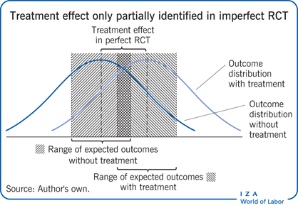
Randomized control trials (RCTs) have become increasingly important as an evidence-based method to evaluate interventions such as government programs and policy initiatives. Frequently, however, RCTs are characterized by “imperfect compliance,” in that not all the subjects who are randomly assigned to take a treatment choose to do so. This could result in a failure to identify the treatment effect, or the impact of the treatment on the population. However, useful information on treatment effectiveness can still be recovered by estimating “bounds,” or a range of values in which treatment effectiveness can lie.
Key findings
Pros
“Partial identification” methods are easy to construct and straightforward to implement in order to estimate causal effects in RCTs with imperfect compliance.
Of particular policy interest is that partial identification methods provide a measure of treatment effectiveness for the entire population.
Partial identification methods require less stringent statistical assumptions than alternative approaches.
Cons
Partial identification does not provide a single prediction but rather a range of values that treatment effectiveness can take.
The range of possible values that treatment effectiveness can take can be sufficiently wide that it is no longer possible to determine whether the treatment has a positive or negative causal effect.
Author's main message
RCTs randomly allocate individuals to treatment or control groups and have become the gold standard of policy evaluation. However, non-perfect compliance in many trials means that comparing the average outcomes for the treated and control populations fails to provide an unbiased estimate of the effect of the policy that is of interest. Instead, only a “partial identification” of possible values of the effect of the policy can be recovered. Even so, this still provides policy-relevant information. Research shows that the methods are simple to implement and are based more on what is known rather than what is assumed.
Motivation
The use of an RCT to determine the causal effect of a treatment or policy can be traced back to work on agricultural experiments in the 1930s [1]. Following the application of RCTs to demonstrate the effectiveness of a new polio vaccine, they gained increasing relevance in drug trials during the 1950s and later became the “gold standard” in medicine.
RCTs have since become increasingly important as an evidence-based method to evaluate many types of interventions, such as government programs and policy initiatives [2], [3]. Within the context of labour markets, RCTs have been successfully used to evaluate the effect of negative income tax and national health insurance policies as well as numerous job-training and welfare programs in the US. They have also been widely used in European countries. The use of data generated from RCTs is increasingly popular among policymakers and practitioners for providing convincing evidence of the causal effect of mandating a social program on various policy outcomes.
However, RCTs are frequently characterized by imperfect compliance, in that the treatment assignment and the actual “take up,” or treatment delivery, are not the same. This could occur when not all subjects who have been randomly selected to take a treatment actually choose to do so, or when those randomly assigned not to take the program decide instead to take it. This results in an RCT with imperfect compliance [4]. Such imperfect compliance results in a failure to identify the point estimate of the treatment effect, i.e. the impact of the treatment on the population, which is what is of most interest to policymakers.
In an imperfect RCT, the causal effect of the policy can no longer be estimated from simply comparing the mean outcomes for the treatment and control groups. This is because outcomes associated with taking or not taking the treatment among subjects who deviate from the random assignment are not known. It is therefore no longer possible to determine the causal effect of the treatment even if the treatment status and outcome of each and every individual in the population is known.
Since imperfect RCTs occur frequently in practice there are a number of strategies that are used to analyse data from such RCTs. The most popular are the use of an intent-to-treat measure and the use of a local average treatment effect. Both of these are causal effects but neither measures the impact of mandating the treatment for the entire population.
Discussion of pros and cons
The rationale for RCTs—a hypothetical example
In order to better understand the rationale and value of an RCT approach, it is worth considering a hypothetical example of a job-training program that provides training only to unemployed workers. Of primary interest in this example is whether or not the program increases employment.
In the absence of an RCT, unemployed workers will simply choose whether or not to take the job-training program (or the “treatment”). If 50% of those who decide to take the program are able to gain employment within three months, while only 30% of those who decide not to take the program are able to do so, what does that imply? Should the conclusion be that the difference in employment across those who decide to take and not take the program (at 20 percentage points) is the causal effect of the program on employment?
The answer would be no, since those who chose to take the training are more likely to be highly motivated, or intrinsically different and, therefore, more likely to become employed, irrespective of whether they took the program. In this case, the 20-percentage-point difference in employment outcomes across the two groups is very likely due to a selection effect and not just due to the job-training program in and of itself.
The conclusion is that it is not possible to determine the causal effect of the job-training program on employment by using this kind of observational data, even if there was information on whether each and every unemployed worker in the population took the program together with their employment outcome.
By contrast, in an RCT, whether or not an unemployed worker takes the job-training program is determined by a randomization mechanism: for example, by the flip of a coin. Given a random sample from the population of unemployed workers, within an RCT any unemployed worker in this sample is equally likely to be allocated, or not, to the job-training program. In other words, the individual would be a part of the treatment group (i.e. allocated to the program) or, alternatively, a part of the control group (i.e. not allocated to the program).
Assuming that 45% of those randomized to take the program (i.e. the treatment group) are able to gain employment within the following three months, and only 35% of those randomized not to take the program (i.e. the control group) are able to do so, then the difference in employment across the two groups, at 10 percentage points, can be attributed to the job-training program itself.
If we were to mandate the same job-training program for all unemployed workers, then employment among such workers would increase by 10 percentage points. This is a causal effect of the job-training program on employment, since by randomizing the treatment (or making it equally likely that a subject is part of the treatment or control group), it is ensured that the treatment and control groups are, ex ante, the same in all respects—other than that the treatment group received the job training and the control group did not.
Measures of causal effects
Intent-to-treat
A frequently used measure of causal effects in an imperfect RCT is an “intent-to-treat” (ITT) measure. This compares outcomes across groups that are randomly assigned the treatment, without consideration as to whether the subjects actually take up the treatment or not. This effectively redefines the objective of the analysis, since an ITT measure is the causal effect of a program that is introduced to the entire population, though subjects retain discretion as to whether or not they actually participate [2].
In the context of the hypothetical job-training program presented earlier, comparing employment outcomes across unemployed workers who were randomized to take the program (irrespective of whether they actually took the program) with those who were randomized not to, will give the ITT estimate. This estimate is the effect of introducing a job-training program for which all unemployed workers are eligible but workers retain discretion in whether or not they take up training. This is an important and interesting estimate in its own right. However, incentives for the unemployed to take up the job-training program can be very different in the field than they are in the RCT. This may happen if the job-training program becomes widely endorsed following the RCT. Policymakers may also be interested in the impact of mandating the job-training program for the unemployed, in which case the ITT measure is of less interest than the causal effect that could be estimated from a perfect RCT.
Local average treatment effect
Another frequently used measure of causal effects in an imperfect RCT is a “local average treatment effect (LATE),” which is the ITT measure divided by the fraction of compliers, i.e. those who comply with the randomization mechanism.
It has been shown that the LATE is the causal effect of a treatment for the complier sub-population, given that a certain set of assumptions has been met [5]. The complier sub-population is the sub-population of subjects who would switch treatment status if the assigned treatment were changed (or who are responsive to the randomization mechanism). This complier sub-population is unobservable as well as assignment dependent (or unstable). It is, therefore, likely to be of less interest to policymakers than a causal effect for the entire population that may be estimated from a perfect RCT.
In the context of the hypothetical job-training program, the LATE gives the causal effect of mandating the program for the complier sub-population amongst the unemployed. There is no a priori reason why a policymaker would be particularly interested in estimating causal effects for this sub-population. Additionally, as with the ITT estimate, this sub-population can be different in the field than in the RCT if the incentives to take up the program change.
Partial identification
Another approach, known as “partial identification,” is the estimation of bounds, or the range of values that the causal effect obtained from a perfect RCT might take [2], [4], [6], [7], [8]. This involves replacing the unknown counterfactuals, or treatment effectiveness among those for whom assigned treatment is different from the treatment actually taken, with a range of values these unknown counterfactuals can take.
The advantage of using partial identification methods is that, unlike the ITT measure, they provide the causal effect of mandating an intervention or program and, unlike the LATE, they provide the causal effect for the entire population of interest. They can also be easily calculated using simple formulas [2], [4], [6], [7], [8].
A formal exposition of partial identification or estimation of a range of values for parameters of interest when point identification fails, was initiated in the late 1980s. Research also provides more recent advances [2], as well as a background literature review of similar ideas going back to the 1930s [9].
Three numerical examples
It is useful to consider again the hypothetical job-training program in some more detail and by using three numerical examples. It is assumed that the employment outcome of each unemployed worker depends on whether this worker took the program and not on whether other unemployed workers took the program. It is also assumed that whether the unemployed worker was assigned to or actually took up the program, as well as whether the worker gained employment within three months, is correctly measured. Finally, it is assumed there are no “defiers,” or unemployed workers who would always do the opposite of what the randomization mechanism instructs them to do.
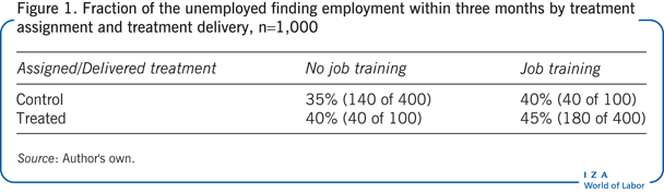
In a random sample of 1,000 unemployed workers, 500 are randomly assigned to take the job-training program and 500 are randomly assigned not to (which is the control group). There is imperfect compliance, so of the 500 assigned to be part of the control group only 80% (or 400) do not take the program while 20% (or 100) decide to take the program instead. Similarly, of the 500 assigned to take the program, only 80% (or 400) actually go on to take the program while 20% (or 100) decide not to take the program. The fraction of workers gaining employment for each group is given in Figure 1.
In order to get a causal effect of the program, it is necessary to compare the fraction gaining employment among those randomized to take the program with the fraction gaining employment among those randomized not to. However, due to non-compliance with the randomization mechanism, it is not possible to obtain a point estimate of this measure.
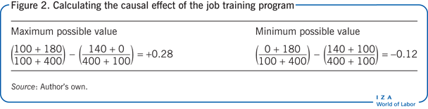
Information about the fraction gaining employment from taking the program among those who were randomly assigned to take the program can be used. However, it is not known how many of the 100 workers who had been randomly assigned to take the program, but who deviated from this assignment, would have been employed had they taken the program. It is known, however, that there can be no fewer than 0 and no more than 100 such workers. Information about the fraction gaining employment from not taking the program among those who were randomly assigned to the control group can also be used. Again, it is not known how many of the 100 workers who were randomly assigned to the control group, but who deviated from this assignment, would have been employed had they not taken the program; however, there can be no fewer than 0 and no more than 100 such workers. The causal effect of the program then takes a maximum possible value of +0.28 and a minimum possible value of –0.12 (see Figure 2).
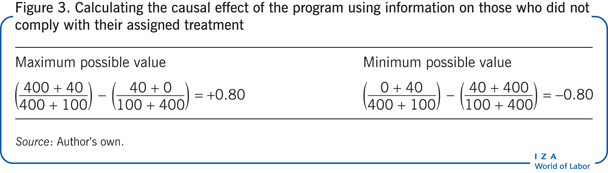
There is also some information about the fraction gaining employment from taking the program using data from those who were randomly assigned to the control group, but who deviated from this assignment to take the program instead. Similarly, there is also some information about the fraction gaining employment from not taking the program using data from those who were randomly assigned to take the program, but who deviated from this assignment to not taking it instead. The causal effect of the program that uses information on those who did not comply with their assigned treatment then compares the fraction gaining employment among those randomly assigned to the control group and the fraction gaining employment among those randomly assigned to the treatment group, which takes a maximum possible value of +0.80 and a minimum possible value of –0.80 (see Figure 3).
The program’s causal effect must simultaneously lie within both the ranges just estimated. Hence, the maximum possible value of the program’s causal effect, which uses all the information generated from this experiment, is the smaller of +0.28 and +0.8, so +0.28. The minimum possible value of the program’s causal effect, which uses all the information generated from this experiment, is the larger of –0.12 and –0.8; hence it is –0.12.
Mandating the job-training program will result in an employment change which may take any value between –12 and +28 percentage points. Since this includes negative as well as positive values, it is not clear whether mandating this program will decrease or increase employment, in the absence of additional assumptions.
The effect of making all unemployed workers eligible for the job-training program with discretion on whether or not the worker chooses to take up this program will increase employment by 8 percentage points. This is the ITT estimate (see Figure 4).
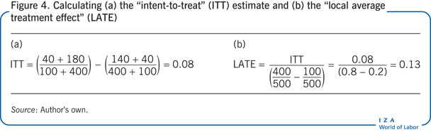
The causal effect of the job-training program for the sub-population of unemployed workers who would switch to taking or not taking the program if assigned to do so by the randomization mechanism is also positive at 13 percentage points. This is the LATE (see Figure 4).
Consider a second configuration of data for the random sample of 1,000 unemployed workers. Suppose the fraction gaining employment within each group is the same as in the first example (now presented in Figure 5), but of the 500 unemployed who are randomized into the control group, just 1% (or 5) choose to take the program instead. Among the 500 unemployed who are randomized into the treatment group, 20% (or 100) choose not to take the program.
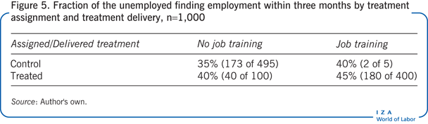
In this case, mandating the job-training program will result in an employment increase between 0.4 and 21 percentage points. Unlike the first example, this example includes positive values for the causal effect only, so the job-training program unambiguously increases employment. The smaller range of values of the causal effect in this case compared to the first is due to fewer workers not complying with the randomization mechanism.
In this example, the effect of making all unemployed workers eligible for the training program, with discretion on whether or not the program is actually taken up, increases employment by 9 percentage points (the ITT estimate). The causal effect of the job-training program for the sub-population of unemployed workers who would switch to taking or not taking the program, if assigned to do so by the randomization mechanism, is also positive at 11 percentage points (the LATE).
Finally, consider a third configuration of data for the random sample of 1,000 unemployed workers. Suppose, in comparison with the second example, that the best employment outcomes or highest fraction gaining employment is among those who were assigned to take the job-training program but who deviated from this assignment, as presented in Figure 6.

In this case, mandating the job-training program for all unemployed workers will result in an employment increase between 0.4 and 21.4 percentage points. The job-training program again unambiguously increases employment.
The effect of making all unemployed workers eligible for the training program, with discretion on whether or not the program is actually taken up, increases employment by 17 percentage points (the ITT estimate). The causal effect of the job-training program for the sub-population of unemployed workers, who would switch to taking or not taking the program if assigned to do so by the randomization mechanism, is also positive at 21.5 percentage points (the LATE).
In this example, both the ITT and the LATE are close to the upper range of values of the partially identified causal effect, with the LATE exceeding the maximum possible value that the causal effect for the population can take. In this scenario, focusing on the ITT and LATE alone would lead a policymaker to over-estimate the potential impact of the job-training program in terms of increases in employment.
Limitations and gaps
While partially identified causal effects in imperfect RCTs make fewer assumptions than alternative approaches, they are not assumption-free.
The hypothetical job-training program presented earlier assumes that the employment outcome of each unemployed worker depends only on whether this worker took the program rather than on whether other unemployed workers took the program. It also assumes that whether the unemployed worker was assigned to or actually took up the program, as well as whether the worker found work within three months, is correctly measured. Such assumptions may be relaxed but they increase complexity in the estimation of partially identified causal effects.
The example assumes that there are no “defiers,” or unemployed workers, who would always do the opposite of what the randomization mechanism instructs them to do; more complex partially identified causal effects have been reported when this assumption is relaxed [6].
Finally, what if a policymaker wants to estimate partially identified causal effects when there is more than one treatment? For example, if there are two different kinds of job-training programs rather than just one. Or a policymaker may want to examine the effect of a program on a continuous outcome, for instance, examining the impact on earnings rather than employment? In such cases, partially identified causal effects may also be estimated but will be more complex [10].
Summary and policy advice
RCTs have become increasingly important as an evidence-based method to evaluate interventions such as government programs and policy initiatives. Frequently, however, RCTs are characterized by imperfect compliance, in that not all subjects randomized to take a treatment choose to do so. This results in a failure to identify the point estimate of the treatment effect, i.e. the impact of the treatment on the population, which is of most interest to policymakers.
In this, as well as other cases in which perfect randomization fails, it is still possible to estimate a range of values in which treatment effectiveness can lie. Within this range any value of treatment effectiveness is as trustworthy as another.
This paper has considered how data generated from an RCT with imperfect compliance can be used to estimate this range of possible values, as well as the pros and cons of this approach compared to alternatives. The advantages of this approach are that it is easy to implement, makes fewer assumptions than alternatives, and provides a causal effect for the entire population of interest. The disadvantage is that the range of possible values for treatment effectiveness may be too wide to give an unequivocal answer as to the direction of the effect (positive, negative, or no effect). Current practice when using data from an RCT with imperfect compliance involves reporting point-identified causal effects such as the ITT or LATE only. However, a more complete picture emerges if estimation of partially identified causal effects were to be carried out on the same data [8].
However, there are pros and cons to the partial identification approach. Partial identification provides a range of possible values for the causal effect of an intervention or program which is mandated for the population of interest rather than point estimates. The range can be sufficiently wide that it is not possible to tell whether the causal effect of the treatment (or a mandatory program) is positive or negative. This is likely to happen, for instance, if a high fraction of subjects do not take the treatment given by the randomization mechanism. In such a case, the “no assumptions” bounds can be narrowed by incorporating additional assumptions that have identifying power. Such assumptions may be motivated by the underlying economic or behavioral model on how potential outcomes vary across those who choose to comply with the randomization mechanism compared to those who do not.
Assumptions may also be made on how potential outcomes vary across observable sub-populations of subjects. For example, that employment outcomes are always higher among those with more years of education. This kind of an assumption could be used to reduce the range of values that the causal effect of the job-training program can take.
In the first numerical example presented earlier, the range of values is sufficiently wide that it is not possible to tell whether the causal effect of the treatment (or a mandatory program) is positive or negative. In the second and third examples, the partially identified treatment effects give a positive causal effect of the job-training program. Examples two and three also indicate that focusing on point estimates such as the intent to treat and local average treatment effect alone would lead a policymaker to over-estimate the potential impact of the job-training program. In short, partial identification represents a comprehensive approach that allows one to examine a menu of causal effects associated with different identifying assumptions as well as how causal effects change as progressively stronger identifying assumptions are included.
The partial identification approach is easy to implement and provides useful information on the causal effect of a policy one could obtain from a perfect RCT. Partially identified causal effects should be reported in order to obtain a better understanding of the impact of mandating a policy when examining data from an imperfect RCT.
Acknowledgments
The author thanks an anonymous referee and the IZA World of Labor editors for many helpful suggestions on earlier drafts. Previous work of the author contains a larger number of background references for the material presented here [8].
Competing interests
The IZA World of Labor project is committed to the IZA Guiding Principles of Research Integrity. The author declares to have observed these principles.
© Zahra Siddique