Elevator pitch
Most of the data available to economists is observational rather than the outcome of natural or quasi experiments. This complicates analysis because it is common for observationally distinct individuals to exhibit similar responses to a given environment and for observationally identical individuals to respond differently to similar incentives. In such situations, using maximum likelihood methods to fit an economic model can provide a general approach to describing the observed data, whatever its nature. The predictions obtained from a fitted model provide crucial information about the distributional outcomes of economic policies.
Key findings
Pros
Maximum likelihood methods enable the measurement of parameters of complex economic models even in the presence of complex sampling schemes.
Maximum likelihood can be used to analyze any kind of data, whether observational, experimental, or quasi-experimental.
By using all the information available in a sample, maximum likelihood methods produce measurements that are as “good as one can get” given the specified model.
Maximum likelihood methods allow the testing of all testable hypotheses that describe a given model.
Cons
Maximum likelihood methods require the specification of an economic model that properly describes the probability distribution of the events observed in the sample.
Using maximum likelihood requires assumptions about the distribution of unobserved components of the model.
If the modeling assumptions are not satisfied, the estimates will suffer from bias, which affects robustness.
Maximum likelihood methods rely on numerical methods to evaluate and maximize the likelihood.
Author's main message
Maximum likelihood is the statistical method of choice for estimating parameters in situations where data are not amenable to the use of statistical techniques that are generally applied to data from experimental studies with a homogeneous population (such as difference-in-differences analysis). A well-specified economic model is a useful tool for understanding the consequences of policy changes that are not necessarily marginal or that affect the distribution of outcomes as well as the mean outcomes. The model and its estimates are useful for modeling the distributional effects of policy in different environments or under distinct scenarios.
Motivation
Much of the recent empirical research in labor economics focuses on the use of field, natural, quasi, or deliberate experiments within a reduced-form framework to identify and measure the causal impacts of economic incentives. This may suggest that progress will come from further exploiting similar methods [1]. Unfortunately for most empirical labor economists, evidence is rarely of this canonical kind: the data may frequently be observational, not experimental, and there may be few, if any, quasi-experimental features that can be exploited. Moreover, it is likely that there are no obvious or convincing instrumental variables available.
Thus, most empirical economists are left to make unpalatable choices: ignore the “wrong kind” of data (observational data) or attempt to recast the data into the acceptable kind, such as by finding a natural experiment to exploit. While attempting to recast the data may occasionally succeed, this approach may not always be possible. Furthermore, in many cases, designing economic policy requires measuring quantities that go beyond the average effect of the treatment on the treated, for example, a wage or an income elasticity. In general, the average treatment effect is likely to be a mixture of parameters that are crucial to the design of a better policy [2], [3].
Economics proposes structural models in which the interactions between observed and unobserved characteristics describe how the data are distributed. Combining structural models with maximum likelihood estimation can provide a useful alternative route to the analysis of both observational and experimental data.
Discussion of pros and cons
Models and data
An estimable economic model makes a number of assumptions about the relationships between variables that describe the environment (exogenous variables) and variables that describe the outcome of interest (endogenous variables). When there are many endogenous variables, the model describes the relationships among them. Finally, the model describes how the variability from uncontrolled sources determines the distribution of outcomes. The precise distribution of outcomes implied by the model depends on the unknown values of particular parameters. The model assumptions can be used to predict the distribution of the observed outcomes in the sample given the exogenous variables and the parameter values, which in turn allows evaluating the likelihood of the data. The purpose of the maximum likelihood estimation method is to find the parameter values that are most likely to generate the observed data: the parameter values that maximize the likelihood of the observed data.
Labor economists already use maximum likelihood methods to estimate parameter values when the conditional distribution of a given type of outcome is well known—discrete (binary, ordered, multinomial, or count models), censored or truncated (tobit models), or selected (Roy model and its generalizations), for example. Most econometric software provides “ready-to-use” estimation routines to obtain parameter estimates for models that fit each particular instance.
In a few cases, where the data are generated through a quasi or natural experiment, the economic model does not have to be fully formulated in order to measure the response of specific outcomes to a given policy change. Nevertheless, such measurements are meaningful only for characterizing the competing models of the world that the analyst considers when analyzing the experiment that generates the data.
The power of economic analysis lies in its ability to clearly state the assumptions about the factors that determine the behavior of agents, given the constraints they face and the assumptions about the mechanisms that allow individual actions to be consistent which each other. For example, in the simplest and most common economic analysis, economists describe a demand curve and a supply curve for a single market and discuss how their interactions determine the equilibrium quantities and prices that are observed.
Models of this type are useful in practice when the analyst is able to distinguish the demand price elasticity (the ratio of the relative change in quantities demanded in response to a 1% change in price) from the supply price elasticity (the ratio of the relative change in quantities supplied in response to a 1% change in price). This is not always possible, however, since the evidence available (equilibrium prices and quantities) is the result of unobserved interactions between the demand and the supply sides. Two strategies are available to make it possible to use observational data to distinguish the behavior of the supply side from that of the demand side: exclusion restrictions, which posit exogenous sources of variations specific to each side, and restrictions on the shape of the demand or the supply schedules, so that the quantity demanded is a decreasing function of the price while the quantity supplied is an increasing function of the price [4]. While one hypothesis may seem more suitable than the other, determining what can be learned from the data requires developing hypotheses that define the critical parameters to be measured.
Richer data require modeling strategies that represent the main features that can be observed. In particular, heterogeneity is an important characteristic of the data labor economists use. It is quite likely in many studies that unobserved/unexplained variability among otherwise similar observations will account for more than half of the observed variability. Having this much heterogeneity that does not correlate strongly with observed characteristic is a feature of data generated by human behavior: even within a homogeneous group of people, the potential variability is large [5]. The hypothesis is that interactions between the determinants of behavioral responses to economic incentives and individual heterogeneity explain the observed features of the data. The measurement of the model parameters may not be amenable to traditional linear regression but may require methods that rely on the distributional characteristics of the data, like the maximum likelihood method.
An illustrative example
An example can make it easier to understand the process of modeling, estimation, and interpretation. Consider a labor supply model for a single worker [6]. The worker will supply labor if the offered wage is large enough; otherwise, they will not participate in the labor market. If this worker supplies their labor, their hourly wage and hours of work per period may be observed. If they do not supply any labor, there are no observable data on the wage that they might have been offered. Thus, individual behavior generates complex data.
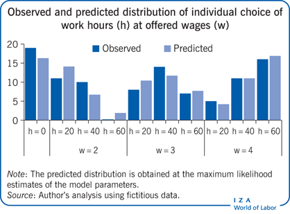
Now consider an imaginary distribution of a random sample of a population of identical individual workers, assuming (to simplify) that three different wage levels are offered and that three positive levels of hours of work are available (see the Illustration). Non-participants are represented by zero hours, and no wage is recorded for them (because observers would not know the offered wage since the job offer was rejected).
Next, a simple labor supply model is fitted to this observed distribution. The model assumes that each individual receives a wage offer (one of the three potential wages) and then decides on the number of hours of work. Individuals are assumed to choose their preferred option by weighing the enjoyment from consuming their earnings against the disutility of work for each alternative level of hours. While the utility of consumption increases with consumption, the marginal disutility of work increases as the time spent at work increases. In addition, there are unobserved components that introduce randomness to the individual decisions: individuals who are observationally identical (in the example, it could be imagined that all individuals in the population have the same age, education, and marital status) can nonetheless exhibit distinct optimal choice (because of personal characteristics that are not observable, such as an individual’s dislike for work). The observed differences in outcomes are thus the result of unobserved differences among individuals. The model depends on three parameters that measure the trade-off between consumption and work as well as the importance of the unobserved component in the distribution of individual choices.
Finally, assume that the probability that a given wage is offered is a single parameter for each wage level and that the process that generates the wage offer and the process that generates individual differences in taste for work are independent (meaning that the observation of the wage offered does not carry any information about the unobserved factors that determine the individual’s choices about work). Therefore, two independent probability parameters characterize the distribution of wages.
The likelihood of the observed sample is then the product over all observations of the probabilities that the hours of work and the wage are observed. For non-participants, the wage is missing and zero hours are observed. The logarithm of the likelihood simplifies the analysis and the search for the parameter values that yield the largest sample likelihood. In this example, it is the weighted sum of the logarithm of the probability of not working and the weighted sum of the summed logarithms of the probabilities of working positive hours for each possible level of hours and for all possible wages.
The need to evaluate and code such an expression is an obvious disadvantage of the maximum likelihood method: in complex cases, it is difficult and time consuming to establish that the log-likelihood is correctly coded. In the current, simple case, the log likelihood is easily maximized using conventional numerical methods (both commercial statistical software and free, open-source math software like R or SageMath supply an optimizer). The Illustration displays the observed distribution of outcomes and the predicted distribution using the maximum likelihood method for the five parameters of the model. The predicted distribution is similar, although not identical, to the observed distribution.
The model for the preferences would yield a labor supply function that takes a simple (log) linear form, such that the logarithm of the hours of work is linearly related to the logarithm of the wage rate. If the observations with zero hours are ignored, the wage elasticity can be estimated by a simple regression over the positive hours (and positive wages) only. The maximum likelihood estimates give an implied elasticity of 2.63, while the regression approach gives an estimate of about 0.66. The difference between the two estimates suggests that the parameter estimates are sensitive to the precise specification of the model and to the sample composition. Since the wage offer distribution and the distribution of the unobserved taste components are independent, the difference between the two estimates arises because of sample selection (the exclusion from the regression estimation sample of the observations for non-participating individuals) and because the observed hours are not determined according to the labor supply function.
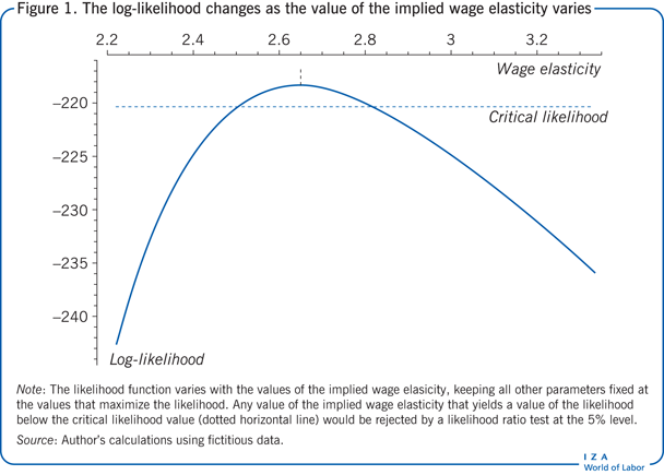
The shape of the log-likelihood describes how precisely the parameters are estimated. Figure 1 shows how the log-likelihood changes as the value of the implied wage elasticity varies, keeping all other parameters at their estimated values. Values of the implied wage elasticity smaller than 2.5 and larger than 2.85 are not supported by the evidence in the data. Furthermore, the 0.66 value obtained by a simple (ordinary least squares) estimation applied to the data with positive hours is far from the maximum likelihood estimate based on the model that accounts for all observations.
Model and policy evaluation
Economic models and likelihood methods can be used together in evaluation studies. Suppose a policymaker wants to understand the labor supply response to the introduction of a minimum wage. The minimum wage does not operate in the first region in either period 1 or period 2, and it operates in the second region only in period 2. Assume, to simplify, that four independent random samples are observed, one for each region and time period, as shown in the upper part of Figure 2. The distribution of the random sample in the second region and in the second period across labor supply and wages after the introduction of the minimum wage is shown in the bottom right part of the table (region 2 in period 2). Each cell in the table reports the number of observations for a given number of hours and wage rate. Non-participants in the labor market (h = 0) do not report their wage, and therefore the number of participants corresponds to h = 0 only and not to a particular wage rate.
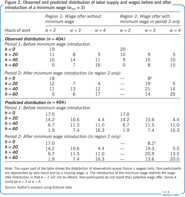
The model assumes that the preferences between work hours and consumption are unaffected by the introduction of the minimum wage; therefore, the preferences are common to all regions and periods. Furthermore, the wage offer distribution with a minimum wage (in region 2) is parametrized independently from the wage offer distribution without a minimum wage (in region 1). This explains why the predicted values for region 1 are the same before and after the introduction of a minimum wage in region 2. Relative to the estimates based on the data described in the Illustration, the behavioral parameters are almost unchanged, while the implied labor supply elasticity is slightly larger, at 2.7.
The evidence for the observed distributions reported in Figure 2 suggests that the introduction of the minimum wage had a sizable effect on the distribution of the hours supplied, in particular, by reducing non-participation in region 2: only eight people are not working (h = 0) in period 2 compared with 20 people in period 1. These distributional changes may not substantially affect the averages and may thus not be captured by a difference-in-differences (DiD) approach, which compares the average change in outcome over time in the case with and the case without the minimum wage, a method that attempts to mimic experimental conditions [7]. But the distributional changes are captured by the fitted economic model, as shown in the lower part of Figure 2: the estimated model predicts a reduction in the number of people who are not working from 17 (without the minimum wage) to 8.2 (when it is introduced).
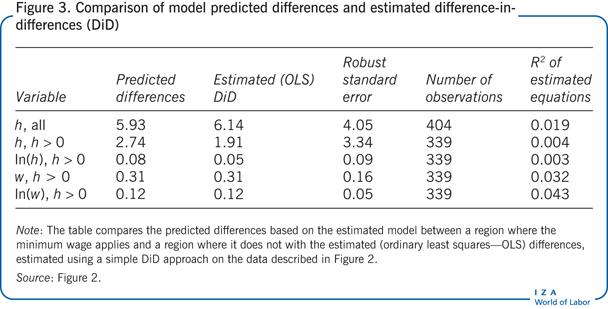
The predicted distribution implied by the model can be used to calculate the effect of the minimum wage, as measured by the DiD approach. The ability to reproduce the results of the less demanding DiD analysis provides a test of the robustness of the model and of the parameter estimates obtained using the maximum likelihood method. The difference in the mean hours of work (or mean positive hours or wage) with or without the minimum wage can be predicted from the specified model. These predicted differences are complex mixtures of the parameters describing the behavioral responses and of the parameters describing the wage offers with and without a minimum wage.
The DiD analysis applied to measure the effect of the introduction of the minimum wage on the hours supplied or wages paid fails to detect any statistically significant (additive) effect on hours, log hours, or wage (when the focus is on positive hours), but it does find a significant (proportional) effect on the average log wage (an increase of about 12%; Figure 3). The predictions reported in Figure 3 from the fitted model and the point estimates from the DiD analysis are in close agreement, which supports the specification of the economic model.
Limitations and gaps
The model in the example discussed above fits the data well because the data structure is relatively simple (in the simplest case, the model needs to predict the probability across only ten cells and does not account for the possibility that the introduction of the minimum wage may reduce the number of job offers received) and because the model depends on a large enough number of parameters (five in the initial case and six when accounting for the effect of the minimum wage). In more realistic and complex situations, it will be harder to understand the features that the model should contain in order to provide a faithful representation of the data and of the mechanisms that generate them. The specification search will include a search for a more flexible representation of the behavioral responses and a search for a parsimonious description of the unobserved variability among individual agents that the model seeks to represent. This search is usually difficult to carry out successfully.
More complex models bring further difficulties when a likelihood-based approach is used. Determining or evaluating the likelihood can be difficult, and numerical issues may arise in seeking to locate the maximum of the likelihood. Such numerical issues can require substantial effort to solve. Often the choice is between a simpler model in which the likelihood estimates are easily obtained and a more complex model in which the estimates are more difficult to characterize or time consuming to obtain.
The specification of a model and the use of a likelihood-based estimation method are not enough to solve the common identification questions that trouble most empirical applications in labor economics. Researchers still need to provide careful arguments for or against the presence of a given explanatory variable in their model.
Summary and policy advice
The use of an economic model and the estimation of its parameters using maximum likelihood can be valuable tools for labor economists. That approach allows for the analysis of data from most sources and can provide insight into the determinants of the usual summary (a parameter estimate in a regression) that a less demanding method, like DiD, will obtain.
Drawing on the example presented in this article, the model could, for instance, be used to calculate a predicted distribution of the population, assuming that the wage distribution is very different, or to assess the effect of the introduction of a minimum wage or an income tax system, assuming that the estimated preferences remain constant. This approach is useful for broader prospective policy analysis. Recent contributions to the literature provide more examples and discussions of the possibilities and difficulties [8], [9], [10], [11], [12].
Finally, the model and the estimates are useful for modeling and understanding the distributional effects of policy in different environments or under distinct scenarios. The illustration of the analysis of the log-likelihood in Figure 1 suggests that such simulation exercises should be carried out over several nearly as likely alternative values for the model parameters. Modern information technology and computer power make the analysis possible for models significantly more complex and valuable than the one presented here. In summary, a methodological approach that uses a model plus maximum likelihood allows for the analysis of a more general class of data (observational as well as experimental) and for a more in-depth analysis of policy design given the parameter estimates.
Acknowledgments
The author thanks an anonymous referee and the IZA World of Labor editors for many helpful suggestions on earlier drafts. Analytical details and calculations supporting this paper can be found on the author’s personal webpage:
Competing interests
The IZA World of Labor project is committed to the IZA Guiding Principles of Research Integrity. The author declares to have observed these principles.
© Gauthier Lanot