Matching as a regression estimator

The LaLonde critique

In 1986, Robert LaLonde published his paper “Evaluating the Econometric Evaluations of Training Programs with Experimental Data” in the American Economic Review [1]. In his paper LaLonde used data from the National Supported Work (NSW) experiment to see if the then standard methods of econometric evaluation could replicate the experimental estimates. Experiments are the most reliable methods of evaluating the causal effect of a certain measure, by comparing individuals who are randomly selected into treatment and control groups, with the only difference between the two groups being that one group receives the treatment and the other does not. In reality, this kind of experimental setting is very rare or even non-existent. However, economic methods aim to deliver the same (causal) results as experiments using different techniques.

LaLonde constructed comparison groups for the NSW experiment from: the Current Population Survey (CPS); and Michigan’s Panel Study for Income Dynamics (PSID). Both are nationally representative samples of the US. The econometric estimators provided estimates that were wildly disparate. Thus, many interpreted LaLonde’s paper as convincingly demonstrating the frailty of econometric models. If no estimate seems to have come very close, can we therefore choose between the various estimators?

Many have interpreted LaLonde’s paper as a damning indictment of the ability of econometric models to provide estimates, but one study notes that many of the estimators that LaLonde considers fail specification tests, which test whether the basic functional form of the model is correct [2].

There are (at least) two possible explanations for the frailty of these models:

• Selection on unobservables: In a non-experimental (real-world) setting, individuals who select treatment (such as, for example, by taking part in additional training) differ in some ways (e.g. ambitions) that are not observed by the researcher (due to missing data, for example) from those who do not select treatment. It is possible that the data are not sufficiently rich to allow traditional methods of estimation.

• Selection on observables and functional form: It is possible that while there may be sufficiently rich data to control for selection, the precise functional form of the regression is not known (e.g. the linear relationship between the outcome of interest—income—and the variable that is expected to explain this outcome, e.g. schooling). This is the argument presented in one particular study, though the analysis used has subsequently been strongly contested [3], [4]. There has been a lively debate between the authors of the studies, the results of which determine whether we may use matching or need to move to models with selection of unobserved variables [5], [6], [7].

  The first explanation regarding selection on observables has sent economists in search of alternative methods of estimation, such as instrument variables, exploiting natural experiments, and, where feasible, conducting social experiments to evaluate programs. The second explanation (natural experiments) motivates us to look at a method that avoids making assumptions about the functional form of the model.

This contribution outlines the conditions that must be in place for researchers to use matching as a tool to answer policy questions.

The evaluation problem

When evaluating social programs, an important objective is to know what impact the program had on each participant. If an individual participates in the program (e.g. training) she might have a different outcome (e.g. higher income) than if she did not. Of course, for each applicant only one of the two outcomes (income with or without training) is observed, giving rise to the fundamental problem of evaluation: only one of the two potential outcomes is observed. The unobserved potential outcome is called the “missing counterfactual.”

The problem of the “missing counterfactual”

If the missing counterfactual could be observed it would be a simple problem, i.e. the impact of treatment would just be the difference in outcomes in the two regimes. But as this is impossible, econometricians try to approach it from a different angle, by looking at the average impact of a treatment. This is easier than finding the treatment effect for every individual.

There are several different average impacts of treatment that might be of interest. Here, the focus will be on two. First, the impact of treatment on the population, or the average treatment effect (ATE), represents the mean (or average) impact of treatment if everyone in the population was treated. That population average is simply the difference in the population averages of the two potential outcomes (i.e. with and without training). However, we may not wish to know what the impact of a program is on the entire population, but are interested more in the impact of treatment on those treated (i.e. the ones who actually participated in the training). This is referred to as the average treatment effect on the treated (ATET).

There is no reason to presume that these two averages are the same. Indeed, most economic models would predict that those who benefit the most are the most likely to participate. Hence, the expectation is that the effect on the treated (with training) is larger than the effect on the total population.

In order to consider how to estimate these treatment effects, it is useful to focus on the effect only on the treated (ATET). The ATET depends on two averages: (1) The average outcome under treatment of those who are treated—which can be estimated from the data; and (2) the (potential) average outcome under treatment of those who are not treated. However, the latter can of course not be observed! This, then, is the “missing counterfactual.”

The problem of the missing counterfactual is not specific to the social sciences. Other disciplines (e.g. medicine) often rely on experiments to solve problems. In an experiment, treatment is allocated randomly. With random allocation of a treatment, the missing outcomes for the treated individuals are equal to the observed outcomes for the non-treated individuals. Thus, in experimental settings the mean outcome of the control group (i.e. those who do not take part in the treatment) will provide a good estimate of the missing counterfactual (i.e. the outcome of the ones who did take part in the treatment given they had not participated). In the social sciences, however, for a variety of reasons it is often difficult to conduct experiments, including ethical concerns. When experiments are not possible, researchers must rely on statistical methods to retrieve the missing counterfactual.

Using OLS regression to estimate the missing counterfactual

Economists frequently use OLS for a variety of estimation requirements, and it is easy to see how it could be used to estimate the missing counterfactual. OLS assumes a linear relationship between the covariates of interest (e.g. education, age, gender) and the mean of the outcome variable (e.g. income). For example, the linearity assumption implies that increasing age by one year changes the mean of the outcome variable by the same amount at ages 20 and 60.

Models from economic theory provide little guidance for the proper functional form (e.g. linearity) that empirical researchers should use. Moreover, the incorrect specification will result in a host of issues that will render the OLS estimates meaningless for estimating the desired causal relationship. In order to overcome this problem, providing there are appropriate restrictions in place, matching can be used to estimate the missing counterfactual. How this is achieved is considered in the following section.

Some assumptions for matching models

Matching is a method that looks at the data to find pairs of individuals who are “identical” except for the fact that one individual participated in the program and the other did not. Not surprisingly, given the considerably weaker restrictions put on the functional form, matching requires other strong assumptions. Unfortunately, one of these assumptions cannot be tested without auxiliary data, while the second assumption is testable. Actually, while it is referred to as an assumption, it is in reality a data requirement in that it forces the researcher to understand the importance of comparing comparable people [8]. While regression will allow researchers to construct the missing counterfactual from very dissimilar people, matching pursues the more conservative strategy of insisting on comparing people that are observationally similar.

Exact matching with discrete covariates

A significant challenge in matching is the estimation of the missing counterfactual in the absence of treatment for every individual who has been treated when the form of the regression function is unknown to the researchers. In order to illustrate this, an example begins with the simplest possible matching estimator, i.e. the exact matching or cell-matching estimator. With this estimator the data are divided into various “cells” that are given all the possible values of X (the explanatory variables). For example, suppose one wants to explain the outcome using the two indicators of gender (male, female) and age (young, old), then one can define four cells (young male, young female, old male, old female). The assumption is that each cell contains treated and untreated individuals.

For each cell, the counterfactual is then the average outcome for the untreated individuals; i.e. the average of the outcomes for individuals who have the same characteristics as the treated individuals but who are not treated. In this example, the missing outcome for young females who received the treatment is then the average outcome among all young females who did not receive the treatment. The conditional independence assumption (CIA) requires the assumption that the outcomes for the untreated individuals in a given cell are equal to the unobserved outcomes in the absence of treatment for the treated individuals. The CIA assumes that, conditional on having the same observed characteristics, receiving the treatment is random. As in the case of a randomized controlled trial (RCT), within a cell, the unobserved outcome for the treated in the absence of the treatment is simply the average outcome observed for the non-treated. The common support assumption (CSA) is needed to ensure that non-treated observations are present to compute the mean outcome for the non-treated. The treatment effect for each cell can now be constructed as the difference in the average outcomes for the treated and for the non-treated.

Of course, there may be a very large number of cells in the data, and examining hundreds or thousands of estimates is not helpful. Therefore the estimates need to be aggregated. The treatment effect is then the weighted sum of the cell effects. The ATET and ATE differ only in the re-weighting of each cell. In the case of the ATET, each cell is given a weight in proportion to the fraction of the total number of treated observed in the cell, while for the ATE each cell is given a weight in proportion to the fraction of the total population in the cell.

Returning to the example, it is assumed that, conditional on gender and age, the allocation to the treatment is as good as random (that is, CIA is invoked), so that the treatment effect in each cell can be computed as the difference in mean outcomes between the treated and the non-treated (see Figure 1).

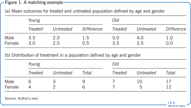
Using the fictional values provided in Figure 1, the mean treatment effect for young males is thus 3.5 – 2.0 = 1.5. Similarly, the mean treatment effects for young females, old males, and old females are 0.5, 1.0, and 0.0 respectively. Figure 1 presents the distribution of individuals across the four groups.

Assuming the following distribution of individuals in the four cells previously defined in Figure 1, the ATET is simply the weighted sum of each cell when the weights are provided by the fraction of the treated population represented by the cell. In the example, the treatment was provided to 10 young and 14 old individuals, so that 24 individuals received the treatment. Young males thus represent 6/24 (25%) of all treated. Similarly, young females, old males, and old females represent 4/24, 7/24, and 7/24, respectively, of all treated. In this example, the ATET is thus as shown in Figure 2.

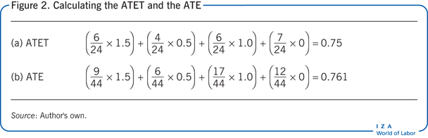
The weights for the ATE are given by the fraction of the population represented by the cell. In the example, the total population is 44, young males represent 9/44 (20.4%) of the population. Similarly, young females, old males, and old females represent 6/44, 17/44, and 12/44 of the population respectively. As such the ATE is computed as shown in Figure 2. Two studies provide empirical examples of the exact matching model [9], [10].

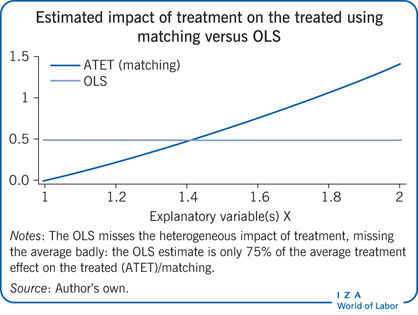
Note that a functional form of the regression function has not had to be specified. This allows the impact of treatment to vary in very complicated ways. The model is both very sophisticated, allowing for complicated patterns in the data, and very easy to estimate. So why would a researcher use OLS?

First, if the OLS equation has been correctly specified, an OLS estimate will have lower variance than the exact matching estimator, such that the estimate received is more precise. Second, some argue that OLS requires “weaker assumptions” than matching. This contains a germ of truth. OLS does not assume the CSA because the assumption about functional form allows for predictions where there are no data. Whether this extrapolation or interpolation to regions without data is accurate or not rests on the ability to correctly specify the functional form. In addition, OLS assumes that the covariates X (explanatory variables) must be orthogonal to the regression error u (i.e. uncorrelated) while matching requires full independence.

The OLS assumption of orthogonality and the matching assumption of conditional independence are both extremely strong and controversial assumptions. Matching affords the researcher the luxury of making no assumptions about the functional form of the regression function, albeit at the cost of using an estimator that can be of a high variance.

Local matching with discrete or continuous data

Exact matching estimators often may have large standard errors because one is relying only on observations that have exactly X = x0 (e.g. age = 34). If there are five observations with age = 34, but four of the observations are in the treated group, an inference is being made about the missing counterfactual with exactly one observation. How, then, might the precision in the estimates be improved?

More concretely, suppose a researcher has matched on a 34-year-old cell and found only two persons in the comparison group. If she looks back to the 33-year-old cell and ahead to the 35-year-old cell, she will find an extra 14 observations. Should those observations be used? Clearly, the estimate of the missing counterfactual will be a much lower variance, because an estimate with 16 observations will have lower variance than one with two observations. More data will generally result in a more precise estimate. But the estimate will be biased because age is only “roughly” 34 (X ≈ x0). Obviously, the reduction in variance is preferable—more precise estimates are preferred to the less precise—but the bias is not considered.

The tradeoff between bias and variance is fundamental to matching. Indeed, with continuous data, there is no choice. Suppose the explanatory variable (age) is continuous and a treated observation with the age of 34 is observed. What is the probability that untreated observations with exactly the age of 34 are observed? Zero. One must take observations with approximately the age of 34. But how far away from 34? The closer one is to 34, the less bias is introduced, but the sample used is smaller and the variance of estimates higher. As observations are selected further and further away from 34, more bias is introduced but the amount of variance is reduced. A “smoothing parameter” therefore needs to be selected that will balance the bias against the variance of the estimator.

How does one select a smoothing parameter to balance this tradeoff between bias and variance? The standard procedure for making that choice is to use a procedure such as “cross-validation” to make out-of-sample forecasts in the comparison sample about the outcome for those who are not treated. The mean squared error of the forecast is then compared across many different possible choices of how close the procedure came to the actual realizations. One then selects the model that best predicts, out of the sample, the outcome for those non-treated individuals. Intuitively, one simply uses all the data, except for one observation, to predict the realization of Y0 (the outcome at age 34) for the observation of interest, which is then compared with the actual realization of Y0. The procedure is repeated for each observation and each value of the smoothing parameter. One then picks the value of the smoothing parameter that minimizes the variance and the sum of the square of the bias.

These methods tend to be computationally intensive and would have been impractical 30 years ago. With the relentless improvement in computational power, these methods can now be implemented on personal computers [11].

Propensity score matching

It would be remiss not to mention the Rosenbaum and Rubin Theorem. This is a remarkable theorem that allows the researcher to match on only one construct, i.e. the probability that the individual is treated. The theorem can be explained as follows: Suppose one has data that satisfy the CIA and the CSA. Then the outcomes with and without treatment are statistically independent of D (another variable), conditional on the probability of treatment for those individuals whose covariates are equal to a specific value.

The theorem tells us that then we need to match only on the probability of receiving the treatment, conditional on the realization of X. Rosenbaum and Rubin call this the propensity score, which is often referred to as propensity score matching. There are two points here that may not be obvious. First, the true propensity score is of course not known. The good news is that it may be estimated [12]. Second, this can reduce the “dimensionality” of the explanatory variables because the propensity score is one-dimensional. This is deceptive, however, because it only pushes the higher dimensional problem back to the estimation of the propensity score. Thus, while the estimation of the matching model has been simplified, it still requires an estimation of the propensity score.

How matching can answer policy questions

While the example used in this contribution nicely illustrates how matching works, it naturally leads to the question of whether a matching estimator could be implemented using real data that answer a substantive question. One study, using the NLSY 1979 Cohort, looked at the return to attending better universities [11]. The study compares the wages of people who attend the first quartile of quality—i.e. the lowest quality university—with people who attend the highest quality. It makes the comparison for men and women separately and compares the matching estimates to corresponding estimates using OLS.

For men, the matching estimates suggest that men who graduate from the best universities earn nearly 15% more than men who graduate from the worst universities. In contrast, the OLS is a 17% wage premium, so the two estimates are pretty close. For women, however, the matching estimate suggests that the wage premium is a little over 8% while the OLS estimate of the wage premium is over twice as high, at nearly 17%.

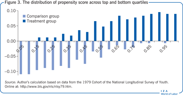
There are at least two reasons for these differences. First, the linear relationship imposed by OLS may be incorrect. Matching, by not imposing linearity, might be more truthfully reporting the true gain to attending elite universities. The second reason, however, has to do with the CSA. Figure 3 plots the distribution of the propensity score across the top and bottom quartiles for women. As is clearly apparent, the wages of women attending lower quality universities are very different from the wages of women attending elite universities, but when the region of common support is observed, the returns to attending elite universities are substantially reduced for women.